My Excel 2016 (2016)
11. Filtering and Consolidating Data
This chapter shows you how to use Excel’s filtering functionality to look at just the desired records. It also shows you how to filter by text, values, and dates. Topics in this chapter include the following:
→ Removing duplicate rows
→ Creating a unique list of items
→ Filtering for specific records
→ Consolidating information from multiple workbooks
→ Filtering a protected sheet
→ Focusing on specific data by filtering by color or icon
Filtering and consolidating data are important tasks in Excel, especially when you are dealing with large amounts of data. The filtering tools can quickly reduce the data to the specific records you need to concentrate on. The consolidation tool can bring together information spread between multiple sheets or workbooks.
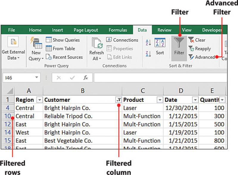
Using the Filter Tool
Filtering allows you to view only the data you want to see by hiding the other data. You can apply a filter to multiple columns, thus narrowing down the data. As you filter the data and rows are hidden, the row headings (1, 2, 3, and so on) become blue.
What’s AutoFilter?
Occasionally, you may see the term AutoFilter used when describing the Filter tool. In older versions of Excel, Excel combined multiple filter tools under the Filter menu, and the AutoFilter was one of them. Now that the tools each have their own button, the old AutoFilter has been simply renamed Filter. But the term still pops up, even in current Excel options.
Apply a Filter
Before you can filter a dataset, you need to turn on the Filter option on the Data tab.
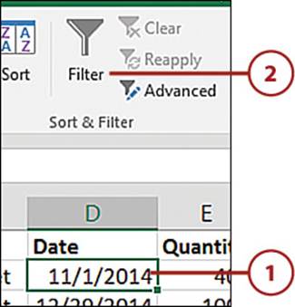
1. Select a cell in the dataset. Excel will use this cell to determine the location and size of the dataset. If you select more than one cell, filtering will be on just for that selection.
2. On the Data tab, select Filter.
Filter Already On for Tables
When a dataset is converted to a table, the headers automatically become filter headers.
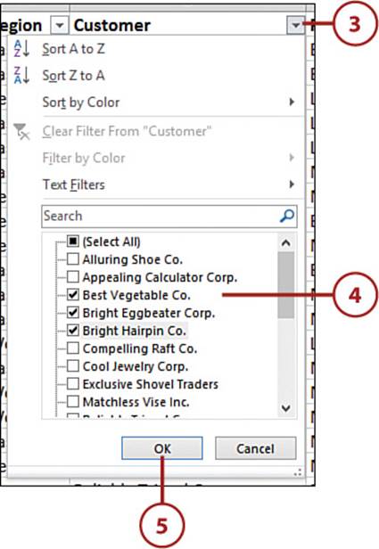
3. Click the drop-down arrow of the column you want to filter.
4. The selected items are the ones that will appear when the column is filtered. Unselect the items you want hidden.
5. Click OK.
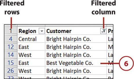
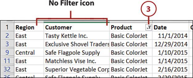
6. The dataset will update, hiding the rows of the items you unselected. Any time you see blue row headings, you know the dataset has been filtered. An icon that looks like a funnel will replace the arrow on the column headers that have a filter applied.
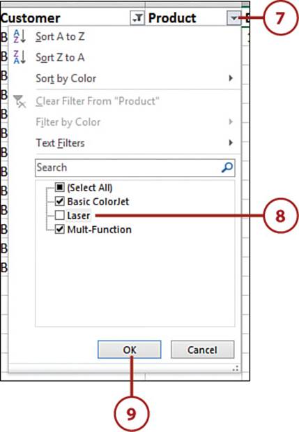
7. Open the drop-down of another column to filter.
8. Unselect the items you want hidden.
9. Click OK.
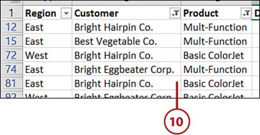
10. Filters are additive, which means that each time a filter selection is made, it works with the previous selection to further filter the data. The dataset now reflects only the records that were selected for both filters.
Turn Filter Off
The Filter button is a toggle button. Click it once to turn filtering on and click it again to turn filtering off.
It’s Not All Good: Excel Didn’t Select the Dataset Correctly
When you apply a filter, Excel will try to help by selecting your dataset for you. You can help Excel do this correctly by not having any blank rows or columns in your dataset. Also, ensure that your header consists of only one row. Only a single header row is allowed—any rows after it are treated as data.
If Excel incorrectly selects your data, turn off the filter, delete the blank columns and rows, and start the previous steps over.
If for some reason you can’t delete the blank columns or rows, you can pre-select the entire table before turning on the Filter functionality.
Clear a Filter
A filter can be cleared from a specific column or for the entire dataset.
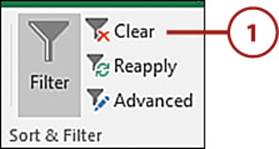
1. On the Data tab, select Clear to clear all filters of the active dataset.
Or
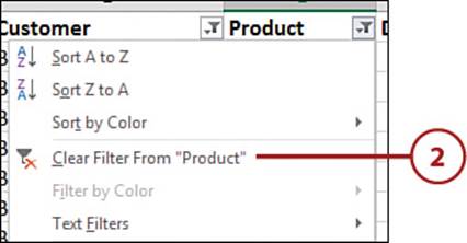
2. To clear a specific column, click the column’s drop-down and select Clear Filter from “Column Header”.
Or
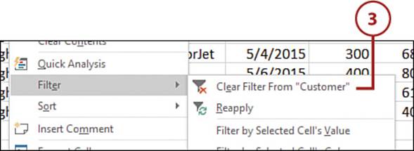
3. To clear a specific column, right-click over the column and from the Filter menu option, select Clear Filter from “Column Header”.
Reapply a Filter
If data is added to a filtered range, Excel does not automatically update the view to hide any new rows that don’t fit the filter settings. You can reapply the filter to work on the extended dataset.
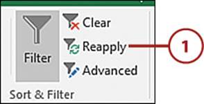
1. On the Data tab, select Reapply.
Or
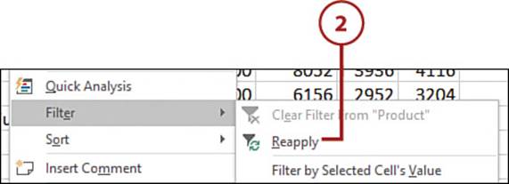
2. Right-click a cell in the filtered dataset and select the Filter, Reapply menu option.
Turn the Filter On for One Column
Filtering can be turned on for a single column or for two or more adjacent columns. Even though you can only select filter items in the columns where the filter drop-downs appear, the filter is applied to the entire dataset.
1. Select the column to turn on the filter for.
2. On the Data tab, select Filter.
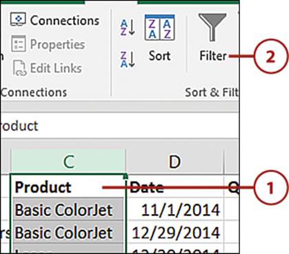
3. The filter drop-down will only be available for the selected column, but will apply the filter to the entire dataset.
Filtering Grouped Dates
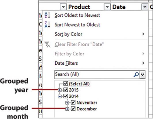
By default, dates in the filter list are grouped by month and year. If you click the + icon by a year, it opens up, showing the months. Click the + icon by a month, and it opens up to show the days of the month. An entire year or month can be selected or unselected by clicking the desired year or month.
Turn On Grouped Dates
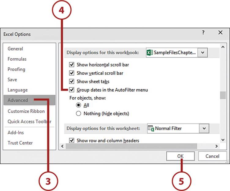
The date grouping is controlled by a setting in the Options menu.
1. Select File.
2. Select Options.
3. Select the Advanced menu.
4. Under the Display Options for This Workbook heading, select the Group Dates in the AutoFilter Menu option.
5. Click OK.
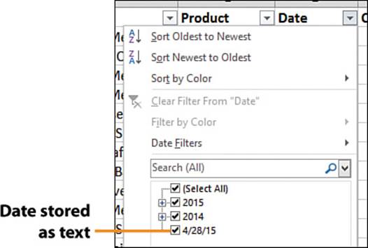
It’s Not All Good: Grouped Dates Still Not On
If the group option is selected and the dates still aren’t grouped (or if you have some dates grouped, but not others), it could be that the dates are formatted as text, not as true dates. See the section “Fixing Numbers Stored as Text” in Chapter 4, “Getting Data onto a Sheet,” for steps to force the dates to be treated as dates.
Filter by Date
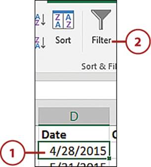
Once the dates are grouped, you can filter for the desired dates.
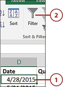
1. Select a single cell in the dataset to apply filtering to.
2. On the Data tab, select Filter.
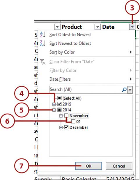
3. Open the drop-down of the date column to filter.
4. Click the + icon to open a group.
5. Click the – icon to close a group.
6. Selecting or unselecting a group parent, such as a month, will affect all the individual items within the group (in this case, the days) the same way.
7. Once the desired filters are in place, click OK. The sheet filters to show only the specified dates.
Using Special Filters
There are other ways to filter the data than by selecting from the list of items. You can filter by color, icon, or selection. Additional filter options are available in the filter drop-down depending on which data type (text, numbers, or dates) appears most often in a column.
Filter for Items that Include a Specific Term
Use the special text filters to select only records that include a desired term.
1. Open the filter drop-down.
2. From the Text Filters menu, select Contains.
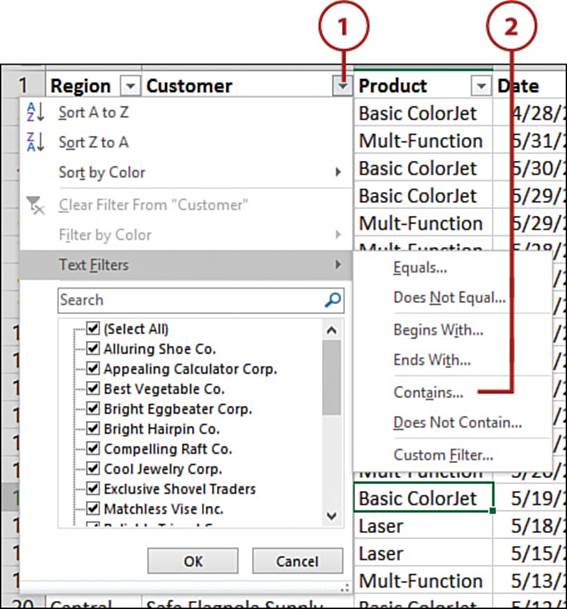
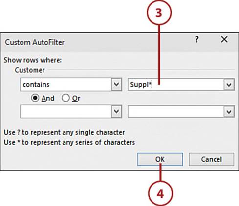
3. Enter the term the cell values should include. Use an asterisk (*) to replace multiple characters or a question mark (?) to replace a single character. For example, to return Supply or Supplies, search for Suppl*.
4. Click OK. The dataset will filter to show the desired records.
Use Conditions in the Custom Filter
The Custom AutoFilter dialog box allows you to combine search criteria. Select the And option if the result must meet both criteria. Select the Or option if the result can meet either or both criteria.
Filter for Values Within a Range
You can filter a numerical column for values that fall within or outside of a specific range.
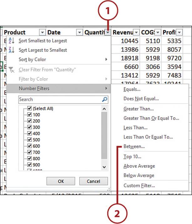
1. Open the filter drop-down.
2. From the Number Filters menu, select Between.
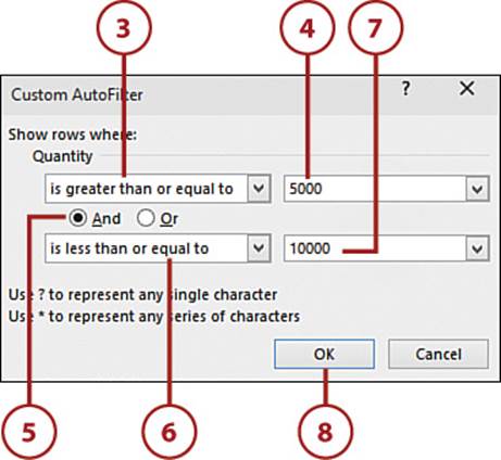
3. Select the desired comparison for the first value.
4. Enter the value.
5. Select And.
6. Select the desired comparison for the second value.
7. Enter the value.
8. Click OK. The dataset will filter to show only those values within the specified range.
Filter for the Top 25 Items
You can filter to show specific records compared to the whole.
1. Open the filter drop-down.
2. From the Number Filters menu, select Top 10.
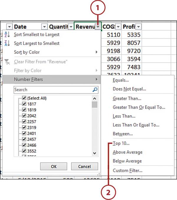
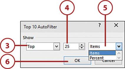
3. Select the desired comparison.
4. Enter the number of top values to include.
5. Choose the comparison type.
6. Click OK. The dataset will filter to show only those values that meet the criteria, in this case, the top 25 items.
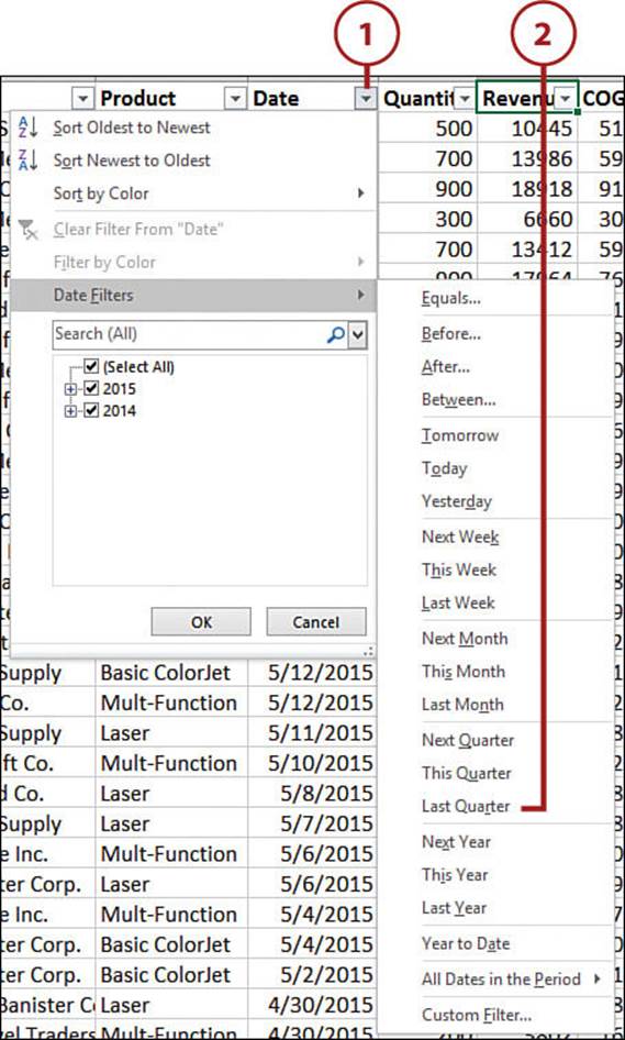
Filter Dates by Quarter
The options dealing with quarters refer to the traditional quarters of a year, with January through March being the first quarter, April through June being the second quarter, and so on.
1. Open the filter drop-down of the Date column.
2. Select a quarter, such as Last Quarter, from the Date Filters menu. The dataset will filter for last quarter’s records.
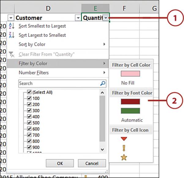
Filtering by Color or Icon
You can filter data by font color, cell color, or icon via the Filter by Color option in the filter listing.
1. Open the filter drop-down of a column with color or icons applied.
2. From the Filter by Color menu, select the desired filter option.
Filtering by Selection
You can filter a dataset without the filter on by right-clicking a cell and choosing to filter by the cell’s value, color, font color, or icon. Doing so will turn on the Filter feature and configure the filter for the selected cell’s property.
Filters are additive, so you can apply more than one using this method, including mixing and matching text and color.
1. Right-click the cell to filter by.
2. From the Filter menu, select Filter by Selected Cell’s Value.
3. Right-click a cell in another column to filter by.
4. From the Filter menu, select the Filter by Selected Cell’s Font Color.
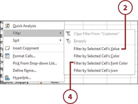
5. The dataset is filtered by the two selections.
Allowing Users to Filter a Protected Sheet
Normally, if you set up filters on a sheet, protect the sheet, and then send it out to other users, the recipients won’t be able to filter the data. But if you set up the protection properly, users won’t be able to modify the data you’ve protected, but they’ll be able to use Excel’s various Filter tools.
Refer to “Protecting the Data on a Sheet” in Chapter 12, “Distributing and Printing a Workbook,” for more information on sheet protection.
Filter a Protected Sheet
Turning on the correct option allows users to filter a protected sheet.
1. Select a single cell in the dataset to apply filtering to.
2. On the Data tab, select Filter.
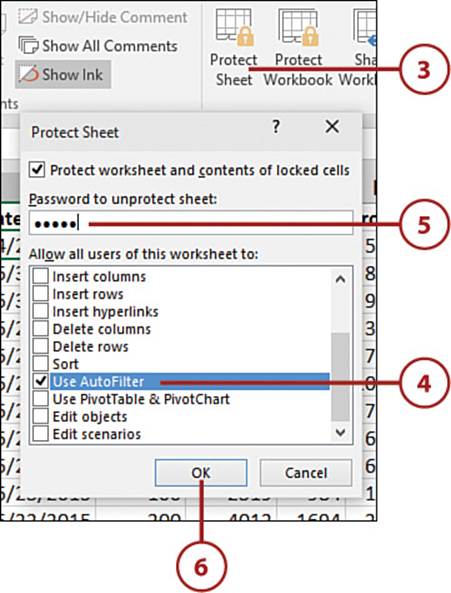
3. From the Review tab, select Protect Sheet.
4. Select Use AutoFilter.
5. Enter a password if desired.
6. Click OK.
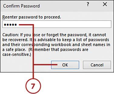
7. If you entered a password in step 5, Excel will prompt you to reenter the password. Do so and then click OK.
Using the Advanced Filter
Despite the visual simplicity of the Advanced Filter dialog box, it can perform a variety of functions, depending on the options selected and the setup on the sheet.
Reorganize Columns
The Advanced Filter can be used to reorganize columns with a few clicks of the mouse. And if this is something you do often, you can set up a template for reuse.
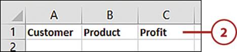
1. Copy the headers from the dataset to a new sheet (the report).
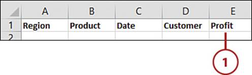
2. Reorganize the copied headers into the desired order. If the dataset has more columns than you need, delete the ones you won’t be needing.
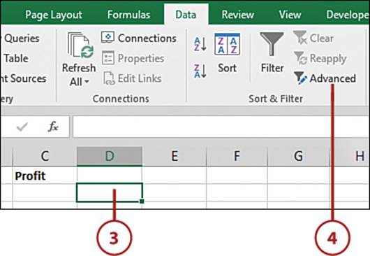
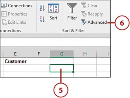
3. Select a cell to the right of the reorganized headers.
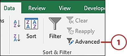
4. On the Data tab, select Advanced.
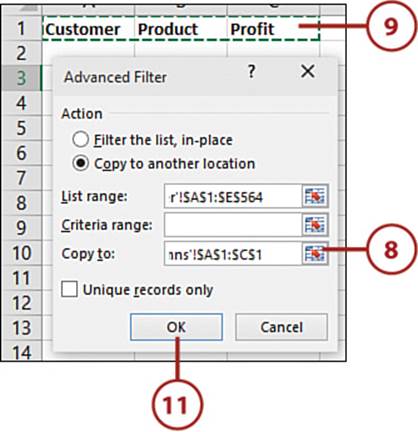
5. Select the Copy to Another Location option.
6. Select the List Range field’s range selector button.
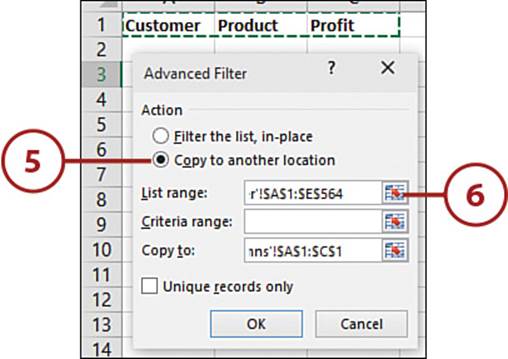
7. Select the entire dataset. Select the range selector button to return to the dialog box.
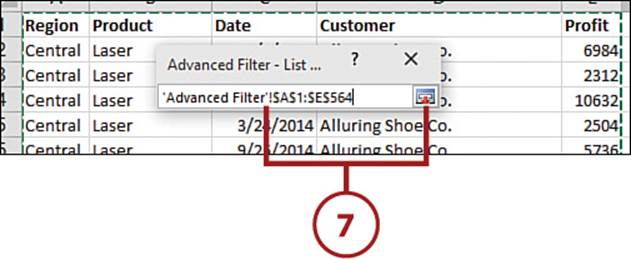
Keyboard Shortcut to Select Dataset
If you’re used to keyboard shortcuts, you may be frustrated that Ctrl+A won’t work in this situation. Instead, select the top-left cell of the dataset, press Ctrl+Shift+Right Arrow, and then press Ctrl+Shift+Down Arrow to select the dataset.
8. Select the Copy To range selector button.
9. Select the headers on the report sheet.
10. Select the range selector button to return to the dialog box.
11. Click OK.
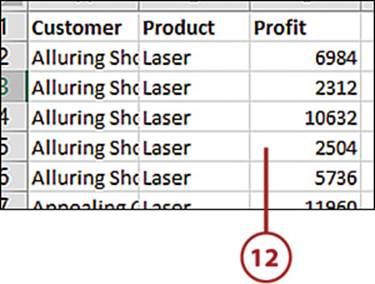
12. The data will be copied to the report sheet. Only the columns with headers will be copied, and in the order you set them up.
Create a List of Unique Items
When the Unique Records Only option is selected, the Advanced filter can be used to remove duplicates. Unlike with the Remove Duplicates command on the Data tab, the original dataset will remain intact if you choose to copy the results to a new location.
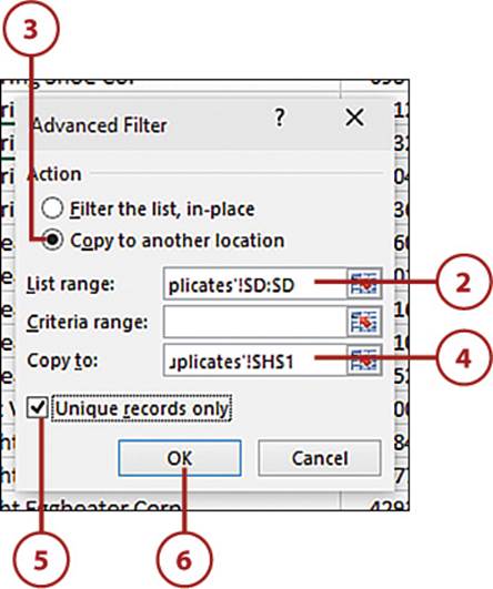
1. On the Data tab, select Advanced.
2. For the List Range field, select the column to create the unique listing from.
Filter the List, In-Place
Select Filter the List, In-Place to only hide the duplicate rows. You can use the Clear button on the Data tab to unhide the rows later.
3. Select Copy to Another Location to place the results in a new location, leaving the original dataset unchanged.
4. Place your cursor in the Copy To field. Select a cell on the sheet for the list to be placed. You cannot place the list on another sheet.
5. Select Unique Records Only.
6. Click OK. The unique list will be created in the selected location.
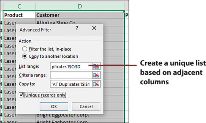
>>>Go Further: Create a Unique List Based on Multiple Columns
You can create a list based on multiple columns if the columns are side by side. The List Range field works only with a single range, but if multiple columns are selected together, they are considered a single range.
The steps are the same as for a single column, but when you’re filling in the List Range field, select all the desired columns.
Filter Records Using Criteria
Criteria are the rules by which you want to execute an Advanced Filter. It’s an optional field in the Advanced Filter dialog box. Criteria can consist of exact values, values with operators, wildcards, or formulas.
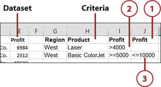
In the following example, we want to create a new report with the following two sets of criteria: Region = West, Product = Laser, Profit > 4000; Region = West, Product = Basic ColorJet, Profit between 5000 and 10000.
1. In row 1 of the dataset sheet, but at least one column away from the dataset, enter the column headers you want to filter on. The text must match exactly, so you may want to copy/paste it. Because the criteria includes a profit range, enter Profit twice.
2. Starting in row 2, enter the criteria. For the first criterion, enter West under Region, Laser under Product, and >4000 under the first Profit column.
3. Enter the second criterion in row 3. Enter West under Region, Basic ColorJet under Product, >=5000 under the first Profit column, and <=10000 under the second Profit column.
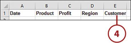
4. Copy the headers from the dataset to a new sheet (the report). You can reorganize or choose the columns filtered over. See “Reorganize Columns” for more information.
5. Select a cell to the right of the headers on the report sheet.
6. On the Data tab, select Advanced.
7. Select Copy to Another Location.
8. Select the List Range field’s range selector button.
9. Select the entire dataset. Select the range selector button to return to the dialog box.
10. Select the Criteria Range field’s range selector button.
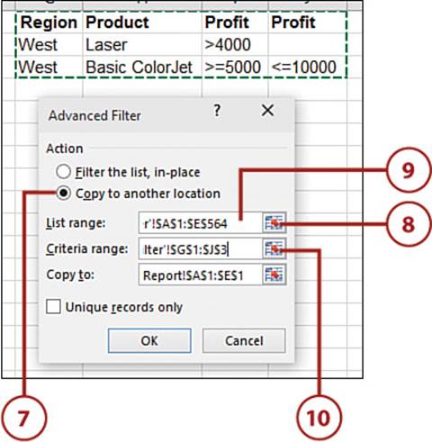
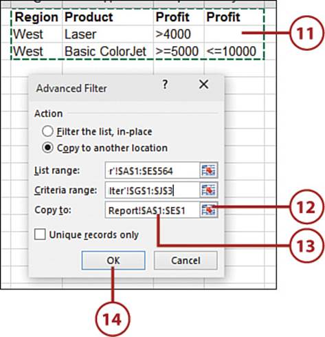
11. Select the criteria, including headers, on the dataset sheet. Select the range selector button to return to the dialog box.
12. Select the Copy To range selector button.
13. Select the headers on the report sheet. Select the range selector button to return to the dialog box.
14. Click OK. The data that fits the two criteria will be copied to the report sheet.
>>>Go Further: Take Criteria to the Next Level
Here are few rules to keep in mind when setting up criteria:
• Criteria entered on the same row are read as joined by AND.
• Criteria entered on different rows are read as joined by OR.
• If a cell in the criteria range is blank and has a column header, this is read as returning all records that match the column header.
• You can have the same header in the criteria twice (for example, if you’re configuring a range).
• If the criteria is for blank cells, enter just an equal sign (=).
• Operators (<, >, <=, >=, <>) can be combined with numeric values for a more general filter.
• Wildcards can be used with text values. An asterisk (*) replaces any number of characters. A question mark (?) replaces a single character. The tilde (~) allows the use of wildcard characters in case the text being filtered uses such a character as part of its value.
Use Formulas as Criteria
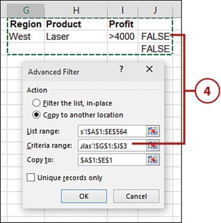
You can combine basic criteria with formulas to create your report. If the criterion is a formula, do not use a column header because the formula is applied to the entire dataset. The formula should be one that returns a TRUE or FALSE value.
For example, you need to create a report of customers in the West region from whom you generated more than $4,000 in profit by selling laser printers. Your data spans a couple of years, so you want to narrow those results down to February and March of the current year. You also want to return any non-West region profits from January of the current year.
1. Set up the basic criteria and report sheet headers as outlined in the section “Filter Records Using Criteria.”
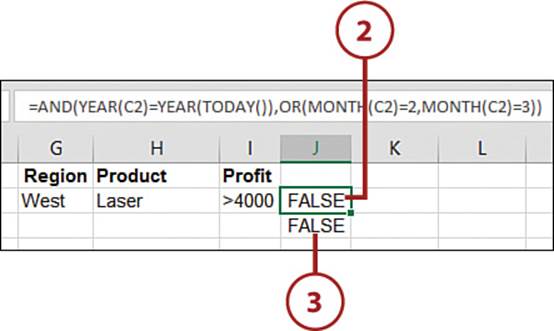
2. In the same row as the criterion for the West region Laser product, enter the formula for the dates. The formula should use relative referencing and refer to the first row of data.
=AND(YEAR(C2)=YEAR (TODAY()),OR(MONTH(C2)=2, MONTH(C2)=3))
3. Enter the second formula in the next row. It also refers to the first row of data.
=AND(A2<>”West”,YEAR(C2)=YEAR(TODAY()),MONTH(C2)=1)
4. Continue with the steps outlined in “Filter Records Using Criteria” to generate the report, making sure to include the formulas when selecting the criteria.
No Basic Criteria, No Problem
If the criteria consists only of formulas and there are no basic criteria with headers, start the formulas in row 2. Also, when selecting the criteria range, include the blank cell in row 1.
Removing Duplicates
The Remove Duplicates tool permanently deletes records from a dataset, unlike other filters, which just hide the rows. The Remove Duplicates dialog box allows you to select the columns to use for finding duplicates.
Delete Duplicate Rows
Because the Remove Duplicates tool permanently removes records from the dataset, you may want to make a backup copy of it.
1. Select a cell in the dataset.
2. On the Data tab, select Remove Duplicates.
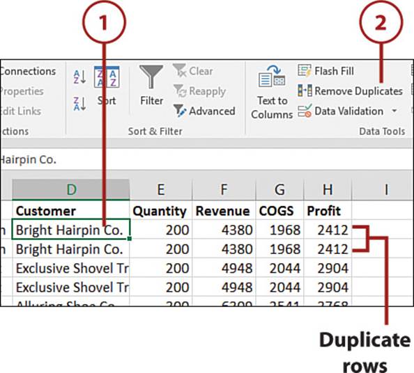
3. Excel will highlight the dataset. If columns are missing in the selection, go back and make sure there are no blanks separating columns.
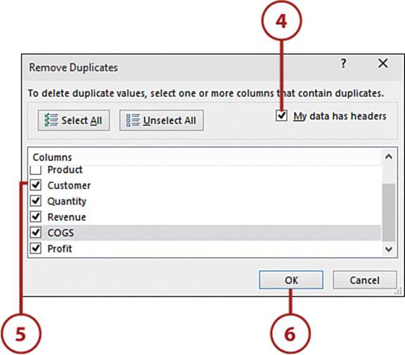
4. If the data has a header row, ensure My Data Has Headers is selected.
5. By default, all the columns are selected. A selected column means the tool will use the column when looking for duplicates. Duplicates in an unselected column will be ignored. In the Columns list box, select the columns to use in the search for duplicates.
6. Click OK.
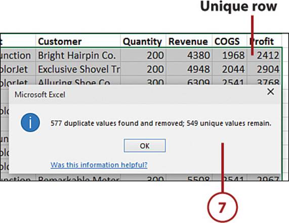
7. The dataset will update, deleting any duplicate rows. A message box will appear informing you of the number of rows deleted and the number remaining in the dataset.
Consolidating Data
The Consolidate tool creates a report of unique records with combined data from different sheets and workbooks.
Merge Values from Two Datasets
You can merge values found on different sheets or in different workbooks based on their relative positions in the selected datasets. For example, if you’re summing the ranges A1:A10 and C220:C230, the calculated results will be A1+C220, A2+C221, A3+C222, and so on.
1. Select the top leftmost cell where the consolidated report should be placed, such as cell A1. If there is other data in the sheet, make sure there is enough room for the new data.
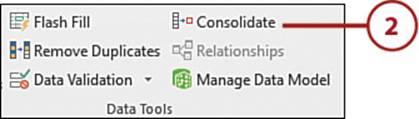
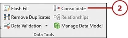
2. On the Data tab, select Consolidate.
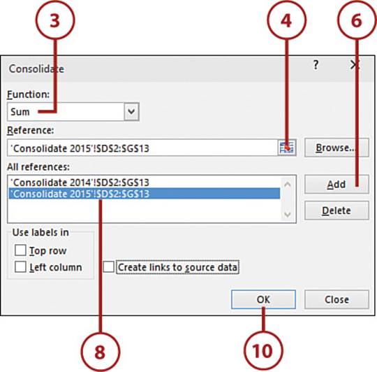
3. Select the desired function.
4. Select the Reference field’s range selector button.
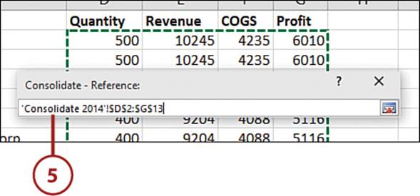
5. Select the first dataset. Don’t select any headers because they won’t be included in the results. Select the range selector button to return to the dialog box.
6. Click the Add button.
7. Select the Reference field’s range selector button.
8. Select the second dataset. Select the range selector button to return to the dialog box.
9. Click the Add button.
10. Click OK.
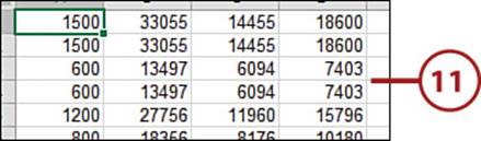
11. The selected calculation will be applied to the corresponding values in each dataset and placed on the report sheet.
Consolidate with a Closed Workbook
If the dataset is in a closed workbook, you can reference it only by using a range name. Click the Browse button to find and select the workbook. After the exclamation point (!) at the end of the path in the Reference field, enter the range name assigned to the dataset.
Merge Data Based on Matching Labels
You can merge values found on different sheets or in different workbooks based on matching row and column labels. If you’re matching row labels, they must be in the leftmost column of the ranges.
1. Select the top leftmost cell where the consolidated report should be placed, such as cell A1. If there is other data in the sheet, make sure there is enough room for the new data.
2. On the Data tab, select Consolidate.
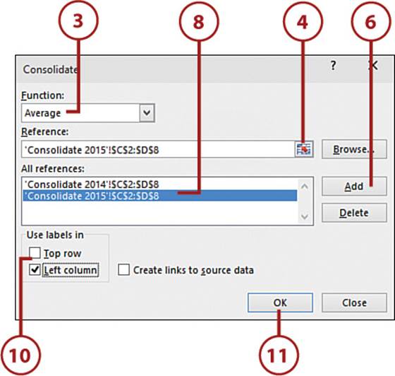
3. Select the desired function.
4. Select the Reference field’s range selector button.
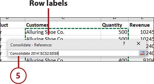
5. Select the first dataset. Include the labels that should be used for the matching. Select the range selector button to return to the dialog box.
6. Click the Add button.
7. Select the Reference field’s range selector button.
8. Select the second dataset, including the labels. Select the range selector button to return to the dialog box.
9. Click the Add button.
10. Mark the Top Row and/or Left Column checkbox(es) to indicate where the labels are in relation to the data.
11. Click OK.
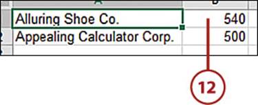
12. Excel will match the labels and apply the selected calculation to the dataset and place the results on the report sheet.
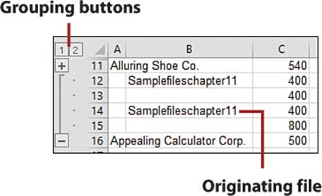
>>>Go Further: Link to Source Data
If Create Links to Source Data is selected, the consolidated data will update automatically when the source is changed. Also, the consolidated data will be grouped. Click the + icon to the left of the data to open the group and see the data used in the summary. If row labels were used to consolidate data, the second column of the report will show the name of the workbook in the first instance of its data.
All materials on the site are licensed Creative Commons Attribution-Sharealike 3.0 Unported CC BY-SA 3.0 & GNU Free Documentation License (GFDL)
If you are the copyright holder of any material contained on our site and intend to remove it, please contact our site administrator for approval.
© 2016-2026 All site design rights belong to S.Y.A.