My Excel 2016 (2016)
12. Distributing and Printing a Workbook
In this chapter, you’ll see how easy it is to leave notes in cells for users, freeze rows and columns so they don’t move as you scroll, and set up a sheet for printing. Topics also include the following:
→ Allowing multiple users access to your workbook
→ Hiding sheets from other users
→ Customizing your page header or footer by adding a logo
→ Printing one sheet or the entire workbook
→ Protecting formulas or text from accidental overwrite
→ Verifying your workbook will work with different versions of Excel
→ Recovering lost data by retrieving a backup file
Once you’re done designing your workbook, you probably want to share it with others. But first, you may want to do a little cleanup, such as adding comments so users can understand what goes in specific fields, hiding sheets you don’t want users to see, or protecting certain cells so users cannot accidently erase your formulas. You can also protect the file so the wrong eyes can’t pry into it.
Once all that’s done, you have to decide how you want to share it. For example, will you print it out, put it on the network and allow multiple users access to it at the same time, or email it? And if you have users with a different version of Excel, such as Excel 2007, you need to ensure those users can access all areas of the workbook without a problem. This chapter shows you how to do this and more.
Using Cell Comments to Add Notes to Cells
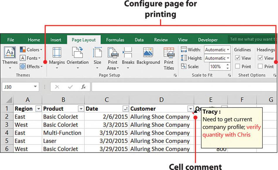
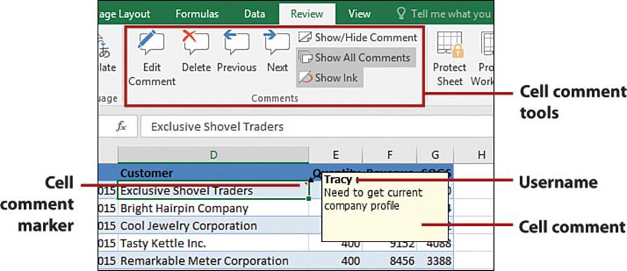
Cell comments are comments or images you can attach to a cell that appear when the pointer is placed over the cell. By default, the cell comment looks like a yellow sticky note. You can tell if a cell has a comment by the red triangle in the upper-right corner of the cell.
Insert a New Cell Comment
Cell comments are a great way to leave a note for other users. For example, you can explain where the value in a specific cell came from or provide instruction on the type of entry expected in a cell.
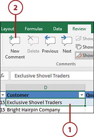
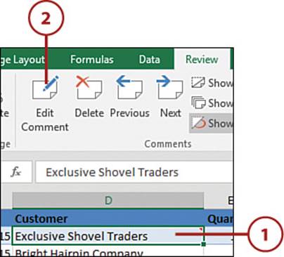
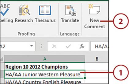
1. Select a cell to which to add the comment.
2. On the Review tab, select New Comment.
Another Way to Insert a Comment
You can also insert a comment by right-clicking over the cell, and selecting Insert Comment.
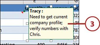
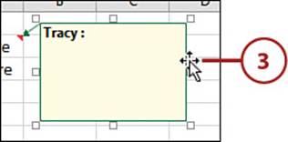
3. Type the desired text. The username is automatically entered by Excel.
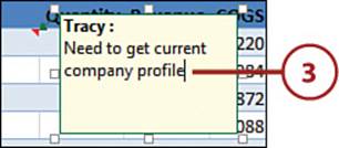
4. Click any cell on the sheet to exit from the comment.
Change the Username
The name shown at the top of the comment is controlled by the username in Excel. This can be changed in the Excel Options dialog box’s General section.
Edit a Cell Comment
Any text in the comment can be edited, including the username.
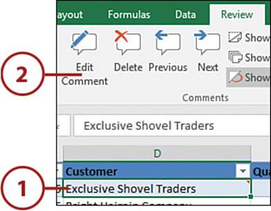
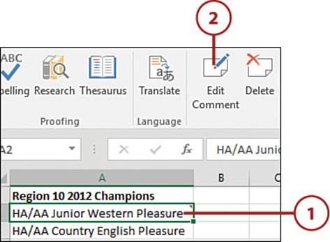
1. Select the cell with the comment to edit.
2. On the Review tab, select Edit Comment.
Another Way to Select Edit Comment
Right-click over the cell and select Edit Comment.
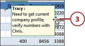
3. Make the desired change to the comment.
4. Click any cell on the sheet to exit from the comment.
Comment Already Visible
If the comment is already visible, just click in the comment box to make changes to the text.
Format a Cell Comment
Once you’ve inserted a cell comment, you can format it.
1. Select the cell with the comment to edit.
2. On the Review tab, select Edit Comment.
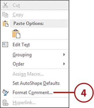
3. Place the pointer on the edge of the comment box so it turns into a four-headed arrow.
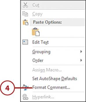
4. Right-click and select Format Comment.
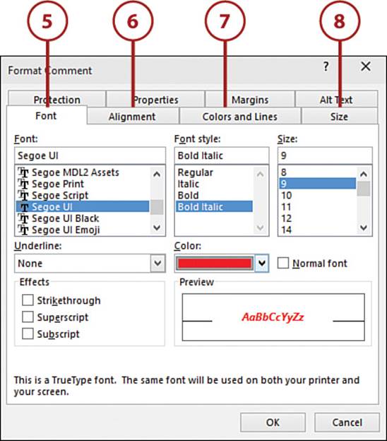
5. Select the desired font styling on the Font tab. Font changes affect all the text in the comment.
6. Change the alignment of the selected text on the Alignment tab.
7. Change the color of the comment box and the frame around it on the Colors and Lines tab.
8. Set the size of the comment box on the Size tab.
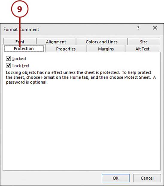
9. Protect the comment box from accidental changes by selecting the check boxes on the Protection tab and protecting the sheet. When selected, the Locked option prevents the comment box from being moved or resized; the Lock Text option prevents the text from being changed.
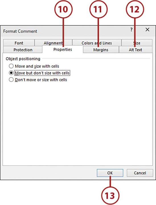
10. Control what happens to the comment box as other cells are sized and moved by choosing the desired option on the Properties tab.
11. On the Margins tab, set the inner margins of the comment box.
12. If you’re going to save the file as an HTML type file, you can enter alternative text for the web browser to display by entering it on the Alt Text tab.
13. Click OK.
Insert an Image into a Cell Comment
You can insert an image into a cell comment as a background fill. The image will take up the entire box and resize as you resize the box. You can still type text in the comment, and it will appear on top of the image.
1. Select a cell to which to add the comment.
2. On the Review tab, select New Comment.
3. Place the pointer along the edge of the comment until it turns into a four-headed arrow.
4. Right-click and select Format Comment.
No Colors and Lines Tab
If the Format Comment dialog box that opens only has one tab (Font), close the dialog box and try again. The dialog box that appears should have multiple tabs.
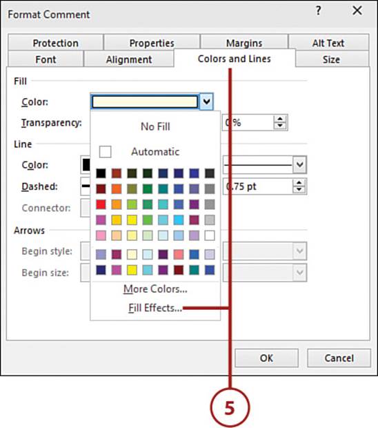
5. On the Colors and Lines tab, select Fill Effects from the Color drop-down.
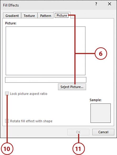
6. On the Picture tab, click Select Picture.
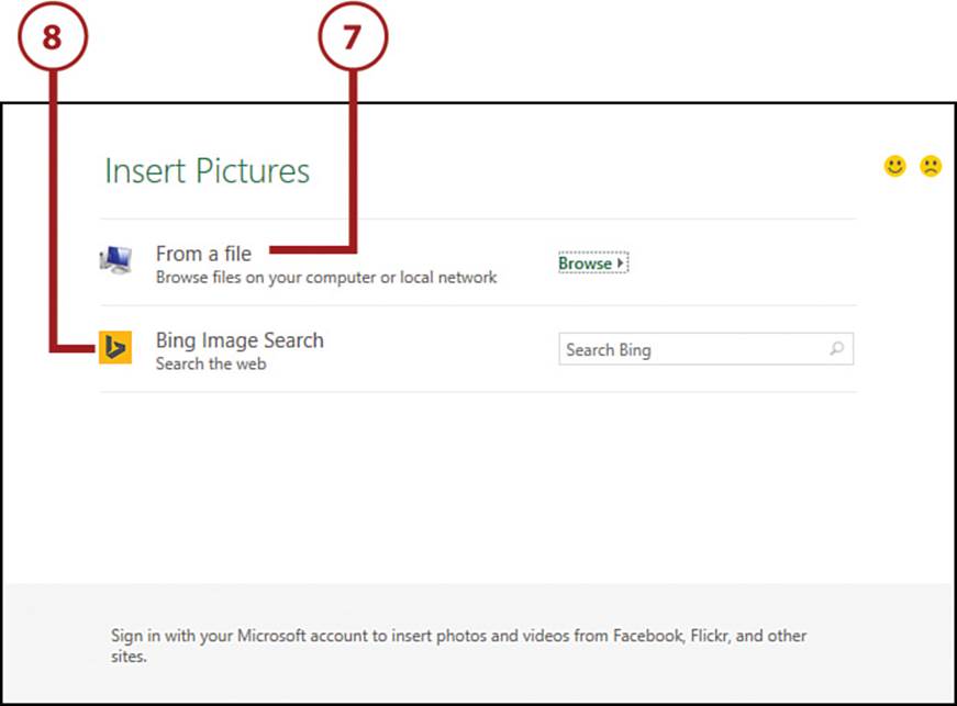
7. Select From a File to browse for the image stored locally, on a network or online drive.
8. Search the Internet for images with a Bing Image Search. Enter keywords in the Search Bing field and press Enter.
Creative Commons
Results returned by Bing may be licensed under Creative Commons. There are different types of CC licenses and you should verify that your usage of the image—for example, if you will be distributing the workbook—falls within the terms of distribution.
More Image Location Options
You might have more image location options listed if you have connected your account to other services, such as OneDrive and Facebook.
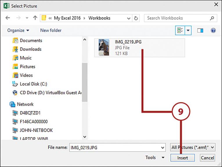
9. Select the desired image and click Insert.
10. Select Lock Picture Aspect Ratio to lock the image ratio.
11. Click OK twice to return to Excel.
12. Use the sizing handles to resize the comment box.
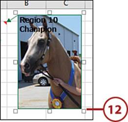
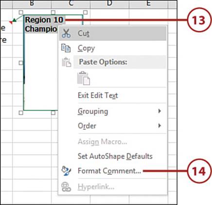
13. When you click in the comment box, the image is hidden so you can see the text. Highlight the text in the comment box.
14. Right-click within the comment box and select Format Comment.
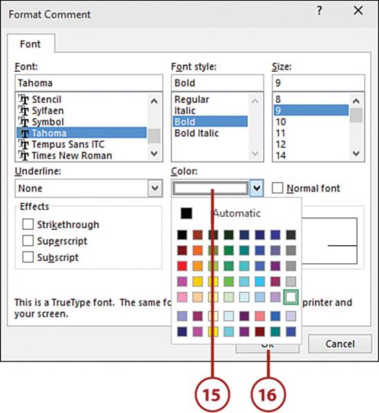
15. From the Color drop-down of the Font tab, select a new color for the font.
16. Click OK.
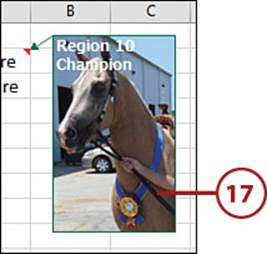
17. Click any cell on the sheet to exit from the comment. Place your pointer over the cell comment to view the image.
Resize a Cell Comment
Resize a comment so all the text or the entire image can be seen.
1. Select the cell with the comment to edit.
2. On the Review tab, click Edit Comment.
3. Click and drag any of the sizing handles (small white squares) around the comment. When the comment is the size you want, release the mouse button.
4. Click any cell on the sheet to exit from the comment.
Show and Hide Cell Comments
A cell comment becomes visible when the pointer passes over the cell and then hides again once the pointer moves away from the cell. You can keep all or some cell comments visible at all times.
1. On the Review tab, select Show All Comments to make all comments in the workbook visible.
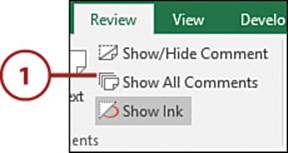
2. If Show All Comments is active, select it again to hide all comments.
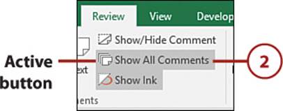
Show All Comments Not Active
If comments have been individually set to be visible, Show All Comments won’t appear active. However, you can still use it to hide all comments by clicking it twice—the first click makes them all visible, the second click hides them.
>>>Go Further: Show/Hide Comments For a Single Cell
You can show/hide the comment of a single cell by selecting the cell with the comment and then using one of these methods:
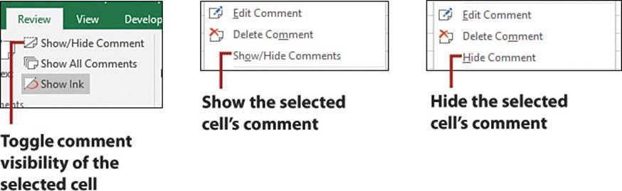
• On the Review tab, select Show/Hide Comment to toggle the comment’s visibility.
• Right-click over the cell and select Show/Hide Comments to make the comment visible.
• Right-click over a cell and select Hide Comment to hide that cell’s comment.
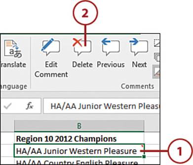
Delete a Cell Comment
Delete a comment to remove it entirely from the cell, including the indicator. If you want to remove the text, refer to the section “Edit a Cell Comment.”
1. Select the cell with the comment to delete.
2. On the Review tab, click Delete.
Another Way to Delete a Comment
Right-click over the cell and select Delete Comment.
Allowing Multiple Users to Edit a Workbook at the Same Time
Excel workbooks are not designed to be accessed by multiple users at the same time. But Microsoft understands that sometimes there is a need for more than one person to edit a workbook at the same time and has provided a limited option.
It’s Not All Good: A Double-Edged Sword
Although Excel allows for multiple user access, what users can do with a shared workbook is severely limited. A shared workbook cannot have tables. Although existing conditional formatting, validation, charts, hyperlinks, subtotals, or scenarios are allowed, new ones cannot be added. Cells cannot be merged and pivot tables cannot be changed. Nor can users write macros or edit array formulas. Basically, only the simplest workbook, such as for data entry, is shareable.
If you need to share a workbook with more advanced options available, such as pivot tables, consider uploading the workbook to your OneDrive. Although not as powerful as the desktop version of Excel, the Excel Web App offers a lot of options. See “Sharing a File Online” later in this chapter for more information.
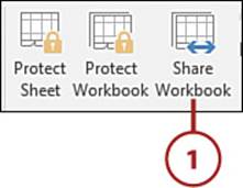
Share a Workbook
You can turn on workbook sharing and save the file to a network location, allowing multiple users to access it.
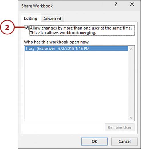
1. On the Review tab, click Share Workbook.
2. Select Allow Changes by More Than One User at the Same Time.
3. Click the Advanced tab.
4. Configure how long the change history should be kept.
5. Choose how copies are updated: when the file is saved or automatically every few minutes.
6. Choose how conflicts should be handled.
7. Select Print Settings if you want users to use their own printings.
8. Select Filter Settings if you want users to use their own filter settings.
9. Click OK.

10. Excel prompts you to save the workbook. Click OK to share the workbook.
Unshare a Workbook
To unshare a workbook, deselect Allow Changes by More Than One User at the Same Time. When you click OK, Excel warns you that the workbook will no longer be shareable, the change history will be removed, and if anyone is currently editing the workbook, changes won’t be saved. If you click Yes, Excel will unshare the workbook and save it.
Hiding and Unhiding Sheets
The option of hiding sheets allows you present a cleaner looking workbook to users—there’s no need for them to see your raw data or calculation sheets.
Hide a Sheet
You can hide sheets you don’t want others to see, just make sure one sheet is left visible.
1. Right-click the sheet’s tab and select Hide.
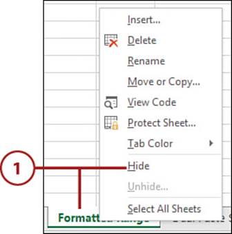
Another Way to Hide a Sheet
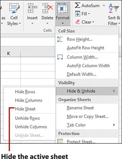
With the sheet you want to hide active, on the Home tab, click the Format drop-down. From the Hide & Unhide menu, select Hide Sheet.
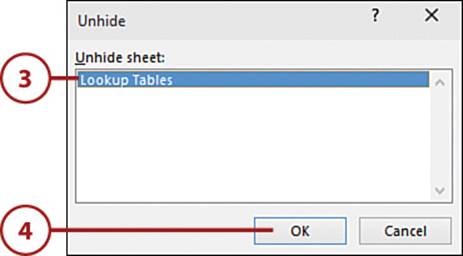
Unhide a Sheet
Unhide sheets when you need to work on them.
1. On the Home tab, click the Format drop-down.
2. From the Hide & Unhide menu, select Unhide Sheet.
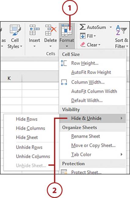
3. Select the sheet to unhide.
4. Click OK.
Can’t Hide or Unhide Sheets
If the workbook is protected (Review tab, Protect Workbook), sheets cannot be hidden or unhidden. See “Set Workbook-Level Protection” later in this chapter for more information.
Using Freeze Panes
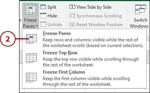
With the Freeze Panes options, you can force the top rows, leftmost columns, or both to remain visible as you scroll around the sheet.
The Table Exception
If you have your data in a table, you don’t need to freeze the top row to keep it visible. Instead, when you scroll the display so that the header row is no longer visible, Excel places the table headers in the headings area for you, replacing the column letters.
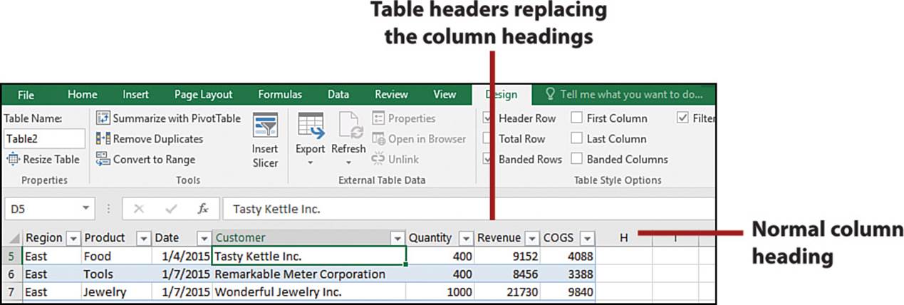
If the headers do not appear in the column headings when scrolling, ensure that you don’t have the Freeze Panes option turned on and that you do have a cell in the table selected.
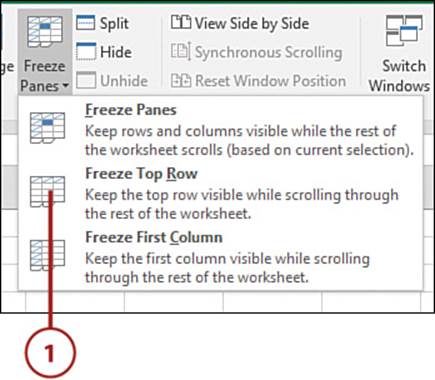
Lock the Top Row
You can lock the first row on a sheet so that, as you scroll down the sheet, you can still see the top row.
1. From the Freeze Panes drop-down on the View tab, select Freeze Top Row.
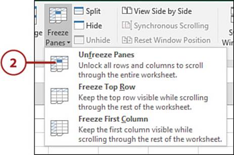
2. To unfreeze the top row, from the Freeze Panes drop-down on the View tab, select Unfreeze Panes.
Lock the First Column
You can lock the leftmost column on a sheet so that, as you scroll across the sheet, you can still see the left column. To do this, select Freeze First Column from the Freeze Panes drop-down on the View tab.
Lock Multiple Rows and Columns
When you use the Freeze Top Row or Freeze First Column option, the selection of one automatically undoes the selection of the other. So, if you want to freeze both the top row and first column, or multiple rows and/or columns, you must use the Freeze Panes option.
1. Select a cell in the row directly below the row and directly to the right of the column you want to freeze.
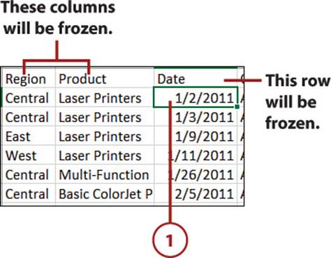
Freeze Rows or Columns, Not Both
If you only want to freeze rows, select a cell in column A; if you only want to freeze columns, select a cell in row 1.
2. From the Freeze Panes drop-down on the View tab, select Freeze Panes.
3. To unfreeze the rows and/or columns, select Unfreeze Panes from the Freeze Panes drop-down on the View tab.
It’s Not All Good: You Can’t Choose What You Unfreeze
If you have rows and columns frozen, you can’t choose to unfreeze one or the other. You must unfreeze them all and then refreeze the part you want to keep frozen.
Configuring the Page Setup
Page setup refers to settings that control how a sheet will look when it is printing. These settings not only include standard print settings, such as the page orientation (portrait or landscape), paper size, and page margins, but they also include settings for repeating rows and columns, printing gridlines, headings, and comments, and more.
Set Paper Size, Margins, and Orientation
You can print your sheet using basic print settings.
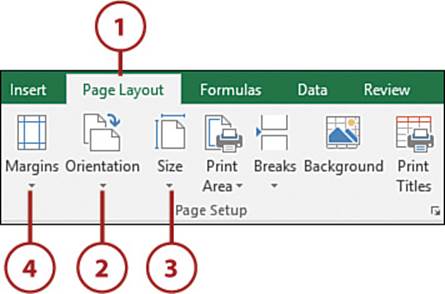
1. Click the Page Layout tab.
2. From the Orientation drop-down, select the page orientation.
3. From the Size drop-down, select a paper size.
4. From the Margins drop-down, select a margin configuration.
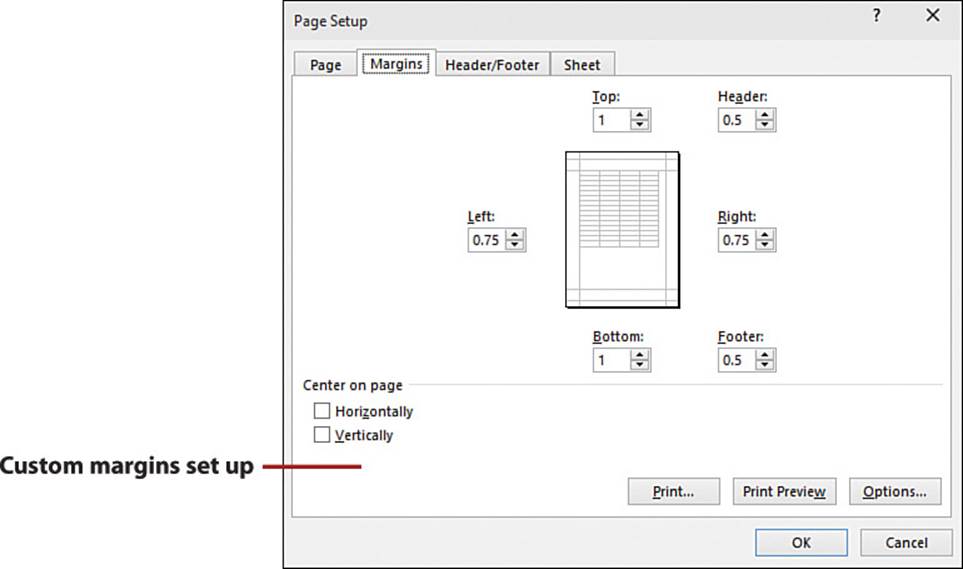
>>>Go Further: Custom Margins
If the margins you need aren’t found in the drop-down, you can set them up. Select Custom Margins from the Margins drop-down to open the Page Setup dialog box, where you can adjust the margins as needed.
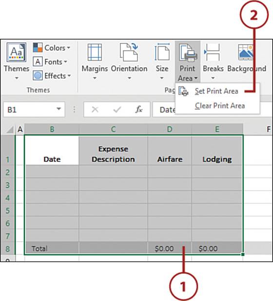
Set the Print Area
The print area is the portion of the sheet that you want to print. By default, it begins in cell A1 and extends down and to the right to capture any cell that has been used, but this can be changed.
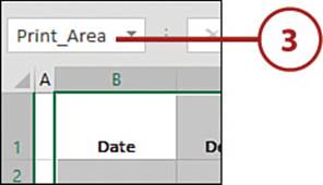
1. Select the range you want to set as the print area.
2. On the Page Layout tab, click Print Area and then select Set Print Area.
3. Print_Area will appear in the Name Box. You can select the name from the drop-down at any time to select (and verify) the print area.
Clear the Print Area
You can reset the print area back to Excel’s suggestion by selecting Clear Print Area from the Print Area drop-down on the Page Layout tab.
Set Page Breaks
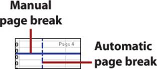
In Page Break Preview, you can see and change breaks. A dashed blue line signifies an automatic page break. A solid blue line signifies a manually set page break.
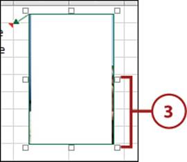
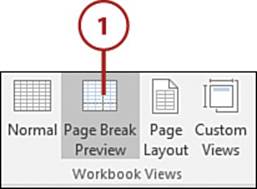
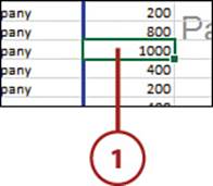
1. On the View tab, click Page Break Preview.
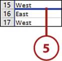
2. To set a horizontal page break, select the row directly beneath the row where you want the page break. For example, if you want the page break after row 15, select row 16.
![]()
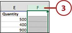
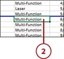
3. To set a vertical page break, select the column directly to the right of the column where you want the page break. For example, if you want the page break after column E, select column F.
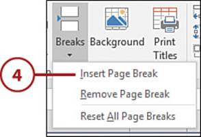
4. On the Page Layout tab, click Breaks and then click Insert Page Break.
5. A solid blue line will appear to show the manually set page break.
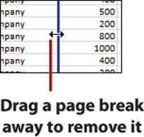
Move Existing Page Breaks
Place the pointer over an existing page break. When it turns into a two-headed arrow, click and drag it to a new location.
>>>Go Further: Delete Page Breaks
You can delete all the page breaks by selecting the Reset All Page Breaks from the Breaks drop-down on the Page Layout tab. You can also remove a specific page break.
1. To remove a vertical page break, select a cell directly to the right of the page break.
2. To remove a horizontal page break, select a cell directly below the page break.
3. On the Page Layout tab, click Breaks and then select Remove Page Break.
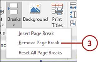
Another Way to Remove a Page Break
Place the pointer over an existing page break. When it turns into a two-headed arrow, click and drag it away from the print area, into the gray area. Note that if you pass over other page breaks, they will also be removed.
Scale the Data to Fit a Printed Page
There are two ways get your data to fit on a page. You can customize the width and height of the data, and you can adjust the scale.
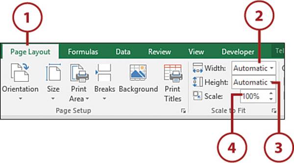
1. Click the Page Layout tab.
2. From the Width drop-down, select the number of desired pages to force a wide table (many columns) to print to fewer pages.
3. From the Height drop-down, select the number of desired pages to force a long table (many rows) to print to fewer pages.
Automatic Width and Height
When the width or height is set to Automatic, Excel sets the page breaks based on the scale, which means your dataset may print out on more than one page.
4. To print the sheet at its actual size, keep the percentage in the Scale field at 100%. The Scale field is used to adjust the scale of the entire sheet. Values less than 100% will reduce the size of the dataset; values greater than 100% will increase it.
Scale Not Available
To adjust the scale, both Height and Width must first be set to Automatic.
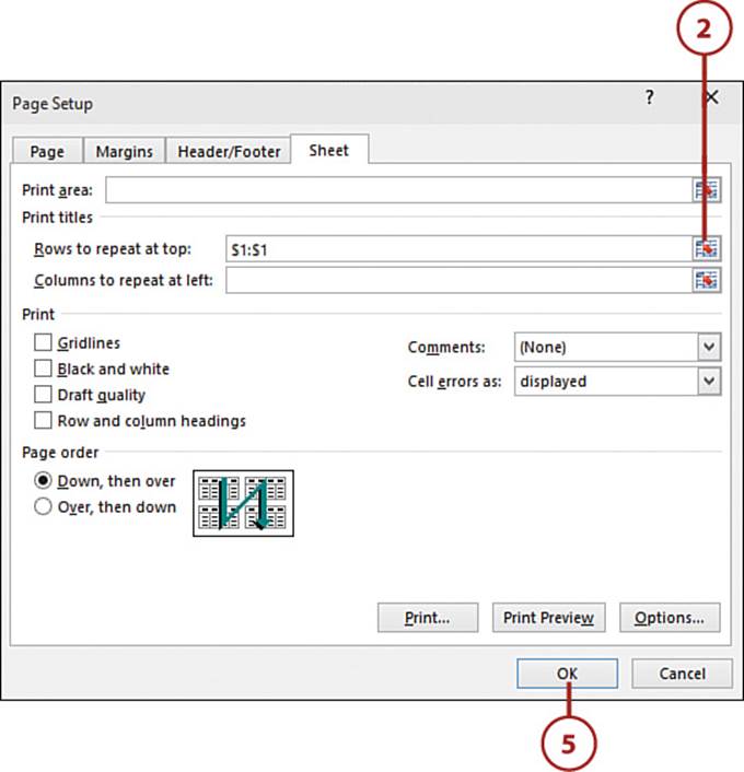
Repeat Specific Rows on Each Printed Page
When you have a report that spans several pages, you can repeat the top rows and leftmost columns on all the printed pages.
1. On the Page Layout tab, click Print Titles.
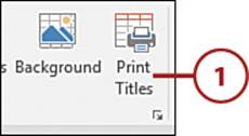
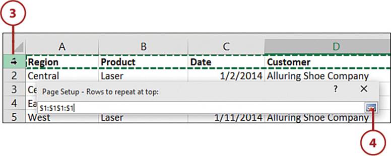
2. Click the range selector.
3. Select the rows to repeat. You can only select the entire row, not just a few columns of it.
4. Click the range selector again to return to the dialog box.
5. Click OK.
Repeat Specific Columns
To repeat specific columns, use the range selector for the Columns to Repeat at Left field to set up the columns. You can only select the entire column, not just a few rows of it.
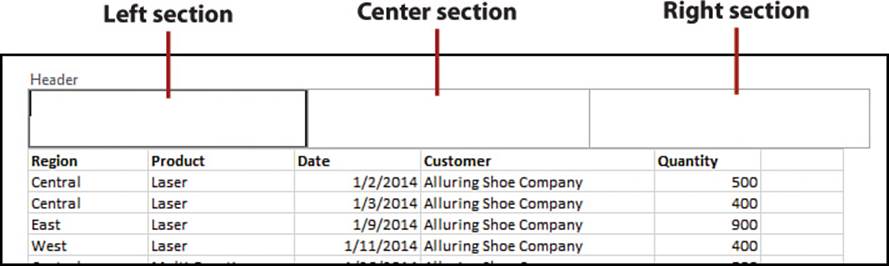
Creating a Custom Header or Footer
The header and footer are unique to each sheet. Each header and footer is broken into sections: left section, center section, and right section. You can customize each of these three sections in the following ways:
• Add page numbering
• Add the current date and time
• Add the file path of the workbook
• Add the workbook name
• Add the sheet name
• Insert text
• Format any text, including the preceding options
• Insert and format an image
Add an Image to the Header or Footer
You can insert one image per section of a header or footer.
1. On the View tab, select Page Layout.
2. Click the section in which you want to place the image, such as the left section of the header.
3. On the Header & Footer Tools Design tab, select Picture.
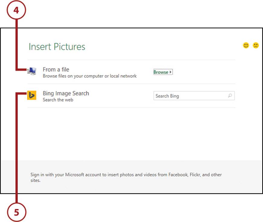
4. Select From a File to browse for the image stored locally, on a network or online drive.
5. Search the Internet for images with a Bing Image Search. Enter keywords in the Search Bing field and press Enter. Note that results returned by Bing may be licensed under Creative Commons.
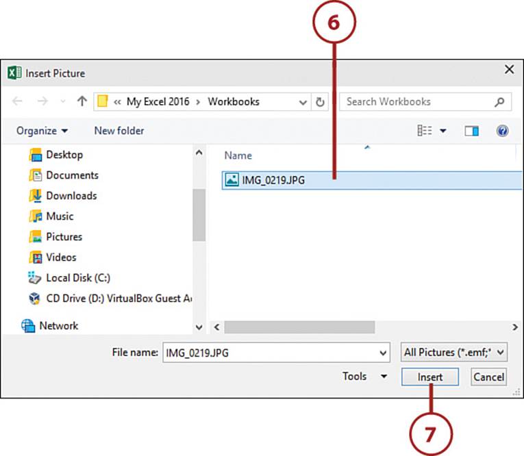
6. Select the desired image.
7. Click Insert.
Not Seeing the Picture
Any time you’re in Edit mode—your pointer is in a section—you will see the code for the picture (that is, &[Picture]). Once you are no longer editing the header or footer, the image will appear.
8. On the Design tab, select Format Picture.
9. Adjust the size of the picture on the Size tab.
10. Click OK.
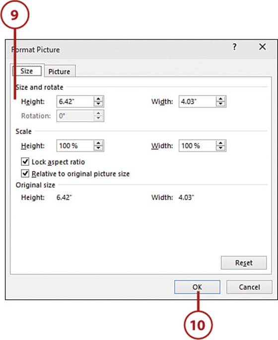
Lock Aspect Ratio
If you know the needed height for the image to fit in the header but not the width, make sure Lock Aspect Ratio is selected before you adjust the height. The width will automatically adjust, preserving the ratio of the image.
11. Click anywhere outside the header or footer, and the image appears. If you need to modify the image even more, click in the section to re-enter Edit mode.
Add Page Numbering to the Header and Footer
You can show just the page number (1, 2, 3, and so on) or you can show the page number out of the total number of pages (1 of 5). If you select multiple sheets when printing, the page numbering will be consecutive for the selected sheets in the order they appear in the workbook.
1. On the View tab, select Page Layout.
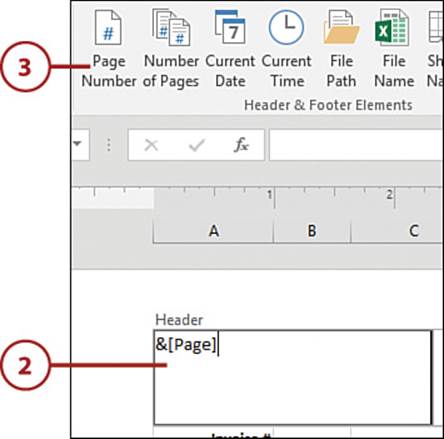
2. Click the section you want to place the page numbering in.
3. On the Header & Footer Tools Design tab, select Page Number to place the page number code (&[Page]) in the section.
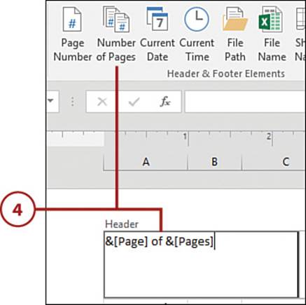
4. To include the total number of pages, type of (with a space on either side of it). Then, on the Design tab, click Number of Pages.
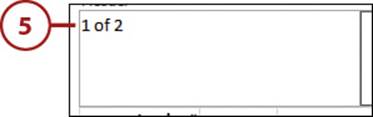
5. Click anywhere outside the footer, and you will see the current page number and the total number of pages.
>>>Go Further: Nonconsecutive Page Numbering
If you don’t want consecutive page numbering across sheets, you need to force the first page number of each sheet.
To do this, go to Page Layout and click the Page Setup group’s dialog box launcher. Near the bottom of the Page tab of the dialog box is a field labeled First Page Number. By default, it is set to Auto, but if you want each page numbering to start at 1 (or another number), you can set the page number here. If you do want the page numbering to be consecutive but it is not, make sure the First Page Number field is set to Auto.
Printing Sheets
Once you’ve configured a sheet for how you want it to print, printing it is easy.
Configure Print Options
Access to various print settings, such as the number of copies and the printer to print to, is available while previewing your sheet. If there’s something you see in the preview that needs adjusting, you can make many adjustments here.
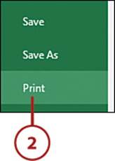
1. Click File to open Backstage view.
2. Select Print, and you’ll enter Print Preview.
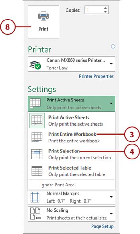
3. To print all visible sheets in the workbook, select Print Entire Workbook from the Print Active Sheets drop-down.
4. To print the selected range of the active sheet, select Print Selection from the Print Active Sheets drop-down.
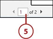
5. On the right side of the screen is a print preview of the sheet. Move through the pages using the scroll wheel of the mouse, the Page Up and Page Down keys on the keyboard, or the arrows at the lower left of the Print Preview window.
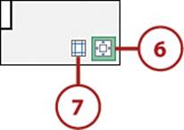
6. Zoom in on the print preview by clicking the Zoom to Page button in the lower-right corner of the Print View window.
7. Click Show Margins to view the margins. You can move a margin by placing the pointer over one and clicking and dragging it to a new location.
8. When the sheet’s page settings are properly configured, click Print to print it.
>>>Go Further: Print Specific Sheets
To print specific sheets, you can hide the sheets you don’t want to print and then use the Print Entire Workbook option. Alternatively, you can use the Ctrl key to select the tabs of the sheets to print. This second method doesn’t require you to select a different print option or hide the sheets, yet it also updates the page numbering.
Protecting a Workbook from Unwanted Changes
After spending time setting up a workbook exactly right, you don’t want another user to mess up your hard work. Or, perhaps your workbook contains sensitive data that should only be seen by certain people. Either way, Excel offers various methods of protection you may find useful.
Set File-Level Protection
Set a password at the file level to prevent an unauthorized user from opening a workbook. You can also allow a user to open the workbook but not save any changes, except as a new file.
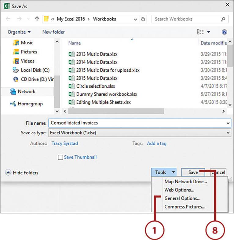
1. In the Save As dialog box, from the Tools drop-down, select General Options.
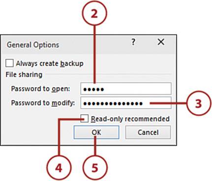
2. Enter a password in the Password to Open field to prevent an unauthorized user from opening the workbook.
3. Enter a password in the Password to Modify field to prevent the user from overwriting the workbook, though it can be saved with a new name or to a new location.
4. If you want to suggest to the user that the file be opened in read-only mode, check the Read-Only Recommended box. Note that this does not force the file to be opened read-only—it is provided as an option.
5. Click OK.
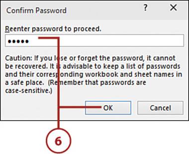
6. If you entered a password for opening the file, enter it again. Click OK.
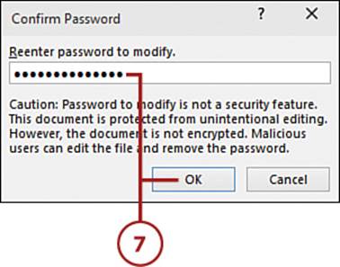
7. If you entered a password for protecting the file from changes, enter it again. Click OK.
8. Click Save.
Remove File Protection
To remove the file protection, return to the General Options dialog box through the Save As option and remove the password. If the file is not read-only, you can overwrite the original file with the new protection settings.
Set Workbook-Level Protection
Protection at the workbook level prevents a user from adding, deleting, or moving sheets.
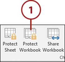
1. On the Review tab, select Protect Workbook.
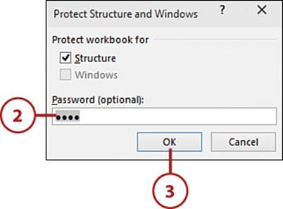
2. If you want, enter a password.
3. Click OK.
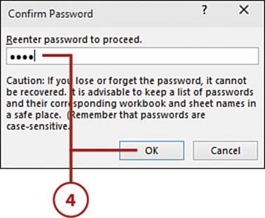
4. If you entered a password, confirm it and click OK.
The Windows Option Is Greyed Out
It’s not a mistake—the Windows option is greyed out and not usable. At the time of writing, it’s no longer an option.
Protecting the Data on a Sheet
Protecting a sheet prevents users from changing the content of locked cells. By default, all cells have the locked option selected, and you purposefully unlock them (see the upcoming section “Unlock Cells”).
Protect a Sheet
Sheet protection must be applied to each sheet individually.
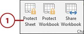
1. On the Review tab, select Protect Sheet.
2. Select what actions a user can take on the sheet. If nothing is selected, the user can only scroll around the sheet. As options in the list are selected, the user can do more, such as enter data in unlocked cells or use the filter drop-downs.
3. Enter a password.
4. Click OK.
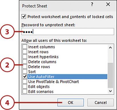
5. If you entered a password, confirm it and click OK.

Unlock Cells
While a sheet is still unprotected, you can unlock specific cells so that when the sheet is protected, users can enter information in those cells. By default, all cells are locked.
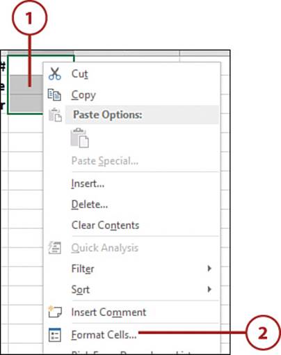
1. Select the cells you want to unlock.
2. Right-click one of the cells and select Format Cells.
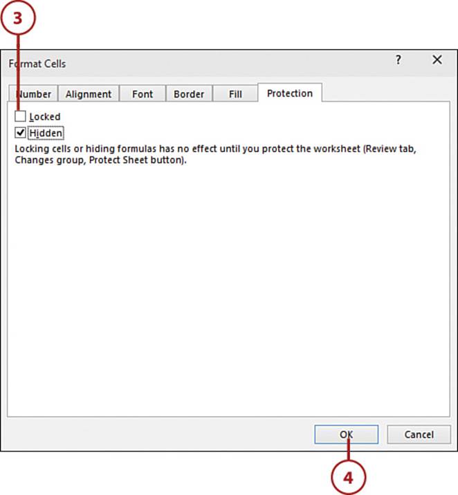
3. Uncheck the Locked option on the Protection tab.
4. Click OK.
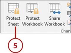
5. Protect the sheet to protect the other cells.
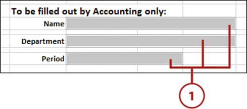
Allow Users to Edit Specific Ranges
Unlocking cells and protecting the sheet is an all-or-none solution. That is, none of your users will be able to modify the protected cells unless they can unprotect the sheet first. The Allow Users to Edit Ranges option lets you assign a password to specific ranges, allowing authorized users to edit those ranges while still protecting the rest of the sheet.
1. Select the cells you want configured for authorized users.
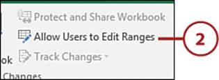
2. On the Review tab, select Allow Users to Edit Ranges.
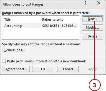
3. Click New.
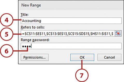
4. Enter a title for the selected range.
5. Refers to Cells should already reflect the cells you want to configure. If not, place your cursor in the field and select the cells on the sheet.
6. Enter the password for editing the range.
7. Click OK.
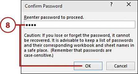
8. Reenter the password to confirm it and then click OK.
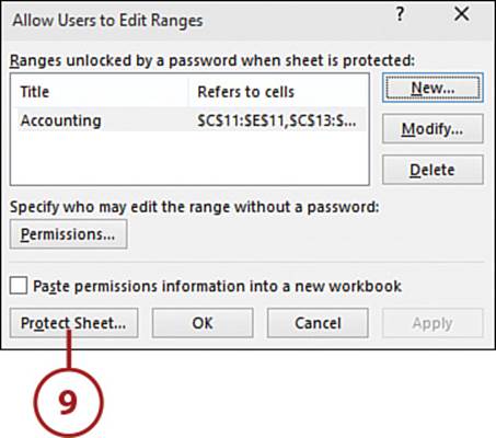
9. Click Protect Sheet.
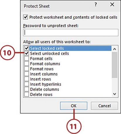
10. Select the option Select Unlocked Cells; otherwise, users won’t be able to select the configured range.
11. Select any other protection options and click OK.
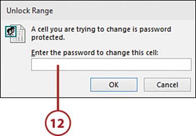
12. The first time a user tries to enter data in the protected range, a password prompt will appear. If the user enters the correct password, the prompt won’t appear again until the workbook is closed and then reopened.
Using the Permissions Option
Clicking Permissions allows you to add users or groups that won’t have to enter a password to edit the protected range. Your network administrator can help you add the correct names.
Edit Allowed Ranges
To edit the allowed ranges, you must unprotect the sheet first.
Preventing Changes by Marking a File as Final
You can inform users a workbook is final and shouldn’t be edited, though the option to edit it is still available.
Mark a Workbook as Final
When you mark as final, the file becomes read-only.
1. Click File to open Backstage view.
![]()
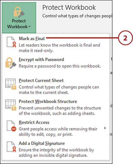
2. On the Info page, select Mark as Final from the Protect Workbook drop-down.
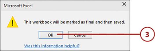
3. Click OK to mark the workbook and save it.
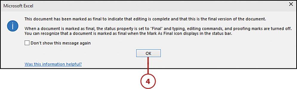
4. Another message box will appear with more information about the final status. Click OK.
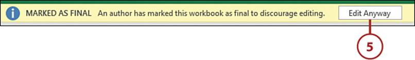
5. The workbook is now marked as final, but a button to edit it is available. If you click the button and save the file, repeat the steps to set the status to final again.
Sharing Files Between Excel Versions
Excel has made many changes over the years. If you plan to send your workbook to users with a version other than Excel 2016, you should ensure that the workbook is compatible with their version(s) of Excel.
Check Version Compatibility
When you check for version compatibility, Excel provides a list of significant and minor issues.
1. Click File to open Backstage view.
![]()
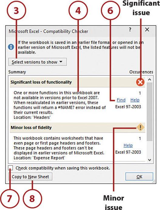
2. On the Info page, select Check Compatibility from the Check for Issues drop-down.
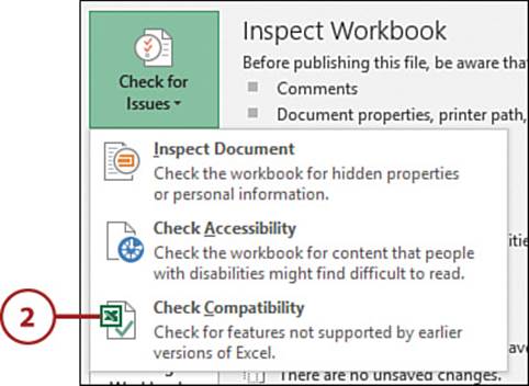
3. Select the version(s) to test for. By default, all versions since Excel 97 are selected.
4. Any compatibility issues are listed with a brief explanation, the versions affected, and whether the issue is significant or minor.
5. If it’s an issue that must be resolved, such as a function not available in previous versions of Excel, click OK, fix the issue, and run the check again.
6. If a Find link appears next to the issue, Excel takes you directly to the issue when you click the link.
7. Select the check box if you want a compatibility check to automatically run whenever the workbook is saved.
8. Click Copy to New Sheet to copy the list of issues to a new sheet in the workbook.
Recovering Lost Changes
Excel automatically creates backups of your workbook as you work on it. Depending on its configuration, it also saves a copy of your workbook if you close it without saving.
Excel won’t keep the auto-recovered files forever. The backed-up copies of the workbook will be deleted under the following circumstances:
• When the file is manually saved
• When the file is saved with a new filename
• If you turn off AutoRecover for the workbook
• If you deselect Save AutoRecover in Excel Options
• When you close the file
• When you quit Excel
Configure Backups
Configure Excel to save backups of your open workbooks. Keep in mind that backing up large files often can slow down Excel.
1. Click File to open Backstage view.
![]()
2. Select Options.
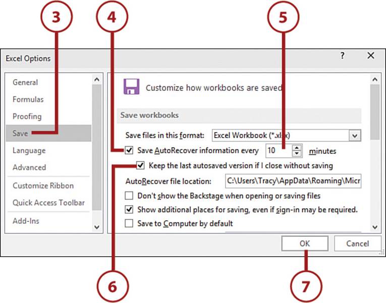
3. Select Save.
4. Select the Save AutoRecover Information Every x Minutes option.
5. Set the number of minutes to a time frame that will work best for all of your workbooks.
6. Select Keep the Last Autosaved Version If I Close Without Saving and Excel saves the last backup copy it made if you close the workbook without saving.
7. Click OK.
Turn Off AutoRecover on Specific Workbook
Turn off AutoRecover for a specific workbook by going to File, Options, Save. Then, under AutoRecover Exceptions For: Current Workbook, select Disable AutoRecover for This Workbook Only.
Recover a Backup
If Excel crashes, you might be able to recover backups of the workbooks that were open at the time.
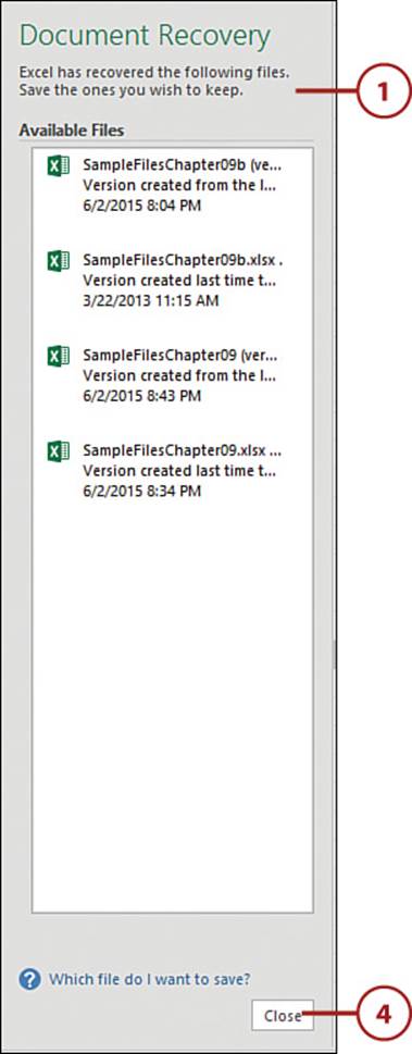
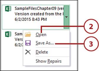
1. If Document Recovery didn’t open automatically when you started Excel, open the original workbook of which you want to retrieve a backup. Document Recovery lists the available backups for the workbook and any other backups it may have.
2. To open a backup, select Open from the drop-down of the desired workbook. If the currently opened workbook has the same name as the backup, it will be closed.
3. To save a unopened backup, select Save As from the drop-down of the desired workbook. The backup will be opened and the Save As dialog box will open. Save the workbook.
4. Click Close to close the Document Recovery window. Any backups that haven’t been opened or saved will be deleted.
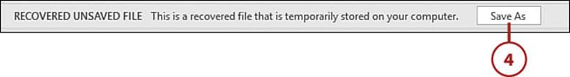
Recover Unsaved Files
If you have a new workbook open long enough for a backup to be created and Excel crashes before you can save it, or you close without saving, there’s a chance you can recover the unsaved file.
1. Click File to open Backstage view.

2. On the Info page, select Recover Unsaved Workbooks from the Manage Workbook drop-down.
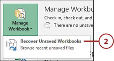
3. Select a workbook and click Open. The workbook will be opened in read-only mode.
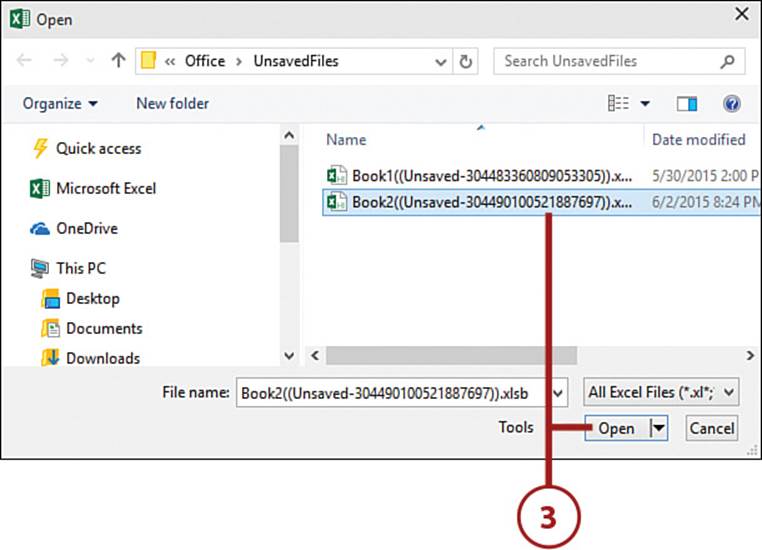
4. To save the workbook, click the Save As button that appears at the top of the sheet. The Save As dialog box will open so that you can save the workbook.
Sending an Excel File as an Attachment
You can email your workbook right from Excel. Excel will open a new message window, attach the workbook, and give you a chance to enter the To and Subject lines and the message body.
Email a Workbook
When emailing a workbook, keep in mind the size of the workbook because different email servers have different size limitations on attachments.
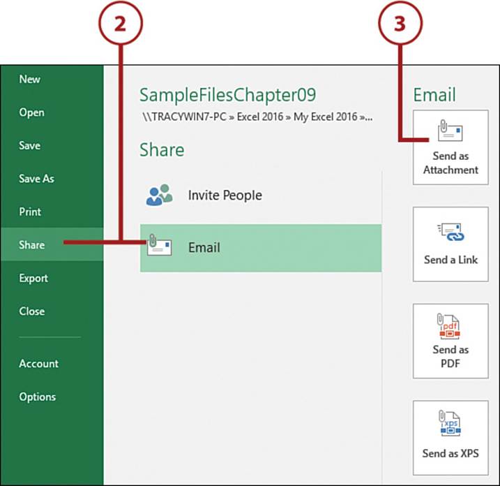
1. Click File to open Backstage view.
![]()
2. On the Share page, select Email.
3. Select Send as Attachment.
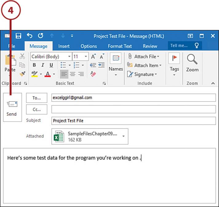
4. Fill in the message fields of the email message and click Send.
It’s Not All Good: Opening Workbooks in Outlook
Outlook gives you the option to open workbooks from within emails. When you do this, a temporary copy of the workbook is created. Because some functionality in Excel requires a properly saved file, you may get errors when you try to work with the workbook. A safe practice is to always save a workbook to your desktop or another location on your hard drive before opening it.
Sharing a File Online
You don’t need to email a file or save it to a network to share it with others. Microsoft offers space on OneDrive, a place online where you can save a file and allow others access.
Save to OneDrive
OneDrive is a free service by Microsoft for storing and sharing files. All you need to use it is a valid Microsoft account. For more information on setting up a OneDrive account and working with online workbooks, see Chapter 17, “Introducing the Excel Web App.”
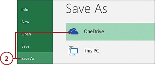
1. Click File to open Backstage view.
2. On the Save As page, select OneDrive.
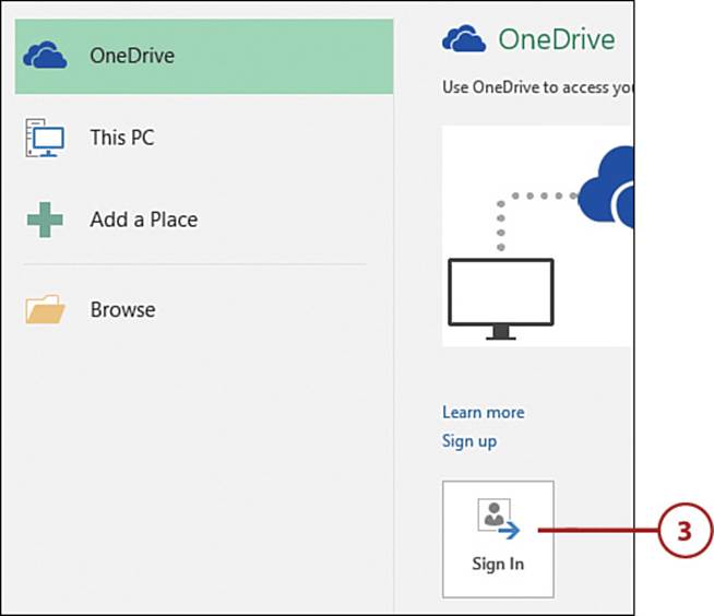
3. If you aren’t signed in to OneDrive, click Sign In. Follow the prompts to sign in to your account. Once signed in, you will be returned to the Save As page. Click OneDrive again.
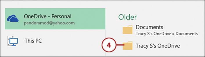
4. Select a folder on your OneDrive.
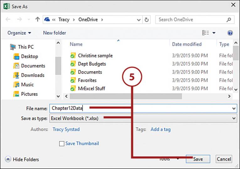
5. Enter a filename, choose a Save As type, and click Save. The file will be saved to your local OneDrive folder and synchronized to the online account.
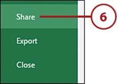
6. Return to Backstage view and click Share.
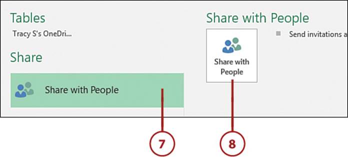
7. If it’s not already highlighted, select Share with People.
8. Click the Share with People button to send an email to those with which you want to share the file. You’ll be returned to your sheet, with the Share task pane open.
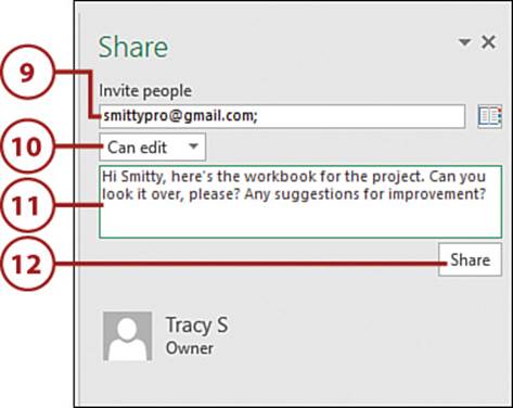
9. In the Share task pane, fill in the recipients’ email addresses. Use a semicolon (;) to separate multiple addresses.
10. Select whether the recipients can edit the workbook or only view it.
11. Enter a message to the recipients.
12. Click Share to send the message. Note that the message is not sent through your local email application but via OneDrive’s online system.
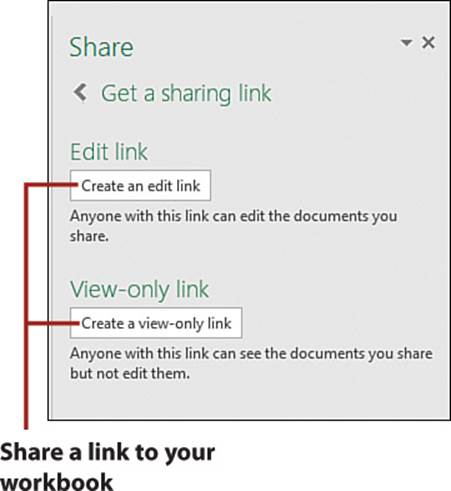
Share a Link
You can also share the workbook by providing a link. Click the Get a Sharing Link in the Share task pane to get a link that you can share any way you please: via email, blog, and so on.
All materials on the site are licensed Creative Commons Attribution-Sharealike 3.0 Unported CC BY-SA 3.0 & GNU Free Documentation License (GFDL)
If you are the copyright holder of any material contained on our site and intend to remove it, please contact our site administrator for approval.
© 2016-2026 All site design rights belong to S.Y.A.