My Excel 2016 (2016)
13. Inserting Subtotals and Grouping Data
This chapter shows you how data can be summarized and grouped together using Excel’s Subtotal and grouping tools. Topics include the following:
→ Manually entering subtotal rows using the SUBTOTAL function
→ Automatically summarizing data using the Subtotal tool
→ Copying just the subtotals to a new sheet
→ Grouping information so you can quickly show or hide data
The ability to group and subtotal data allows you to summarize a long sheet of data into fewer rows. The individual records are still there, so you can unhide them if you need to investigate a subtotal in detail.
Using the SUBTOTAL Function
The SUBTOTAL function ignores the values of other SUBTOTALs within the assigned range, which means your calculated value won’t get doubled. It also calculates the range of numbers based on a code used in the function. With the correct code, SUBTOTAL can calculate averages, counts, sums, and more. It can also ignore hidden rows when the 100 version (101, 102, and so on) of the code is used. The syntax of the SUBTOTAL function is as follows:
SUBTOTAL(function_num, ref1,[ref2],...)
Calculate Visible Rows
Most functions will calculate all values in its range, whether they are visible or not. If you want to ignore the hidden values, use the SUBTOTAL function with the 100 version of the desired calculation code.
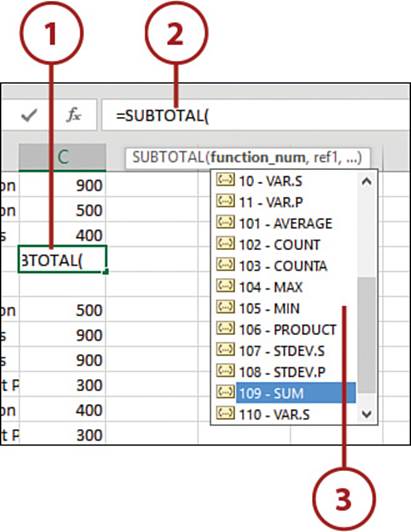
1. Select the cell for the formula.
2. Type =SUBTOTAL(.
3. A drop-down of the various codes appears. The first 11 are like their corresponding functions. For example, 9 - SUM will sum all values. Scroll down to see the 100 codes that calculate only the visible cells. Select the desired code and press Tab, or double-click it.
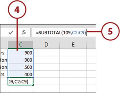
4. Type a comma to move over to the next argument and then select the range to calculate.
5. Type the closing parenthesis and press Enter or Tab to calculate the formula.
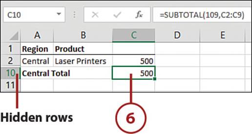
6. Hide some rows in the range. The value will update to reflect the visible cells only.
Summarizing Data Using the Subtotal Tool
The SUBTOTAL function is useful, but if you have a large dataset, it can be time consuming to insert all the total rows. When your dataset is large, use the Subtotal tool on the Data tab. This tool groups the sorted data, applying the selected function.
The Table Limitation
You cannot use the Subtotal tool on a range that has been converted to a table.
Apply a Subtotal
Applying subtotals to a dataset is quick and easy when using the Subtotal dialog box. Because Excel will group the subtotals based on the changing data in the column you select, you need to sort the data in that column first.
Refer to Chapter 10, “Sorting Data,” for more information on sorting.
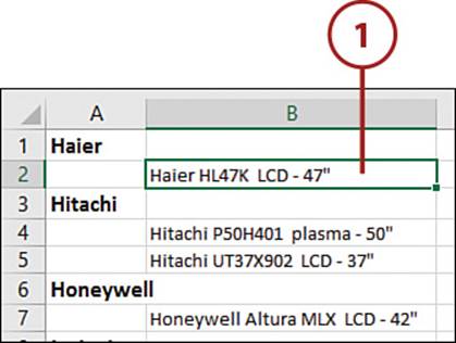
1. Sort the data by the column on which the summary should be based.
2. Select a cell in the dataset.
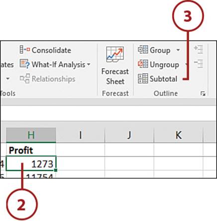
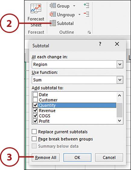
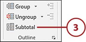
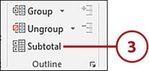
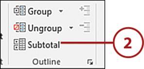
3. On the Data tab, click Subtotal.
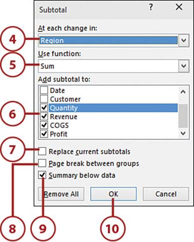
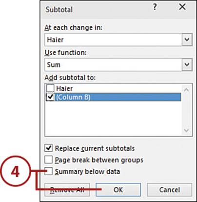
4. Select the column by which to summarize the data—the same column you sorted the data by in step 1.
5. Select the function by which the subtotals will be calculated.
6. Select the column(s) to which the subtotals should be added.
7. Check Replace Current Subtotals if subtotals are already in the dataset and you want to replace them.
8. Check Page Break Between Groups if you want to print each subtotaled group on its own page.
9. Select Summary Below Data to place the totals below each group. Uncheck the box if you want the totals above the group.
10. Click OK. The data is grouped and subtotaled, with a grand total at the very bottom (or top, if that’s what you configured).
Subtotal by Multiple Columns
To subtotal by multiple columns—for example, to sum the quantity of each product within a region—sort the dataset by the desired columns and then apply the subtotals, making sure Replace Current Subtotals is not selected. The sort and subtotals should be applied in order of highest level (Region) to lowest level (Product).
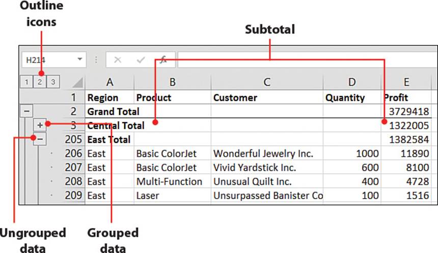
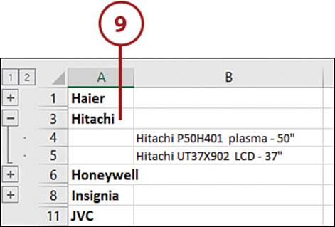
Expand and Collapse Subtotals
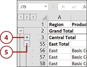
Use the outline symbols to the left of the data to expand and collapse the subtotaled data. The numbers represent the subtotal levels in the dataset.
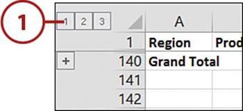
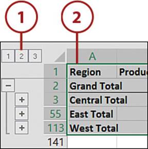
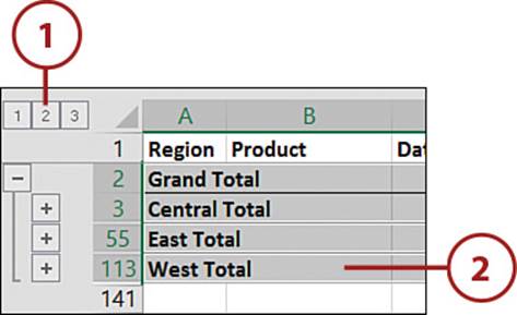
1. Click 1 to view only the Grand Total.
2. Click 2 to view the first level of subtotals.
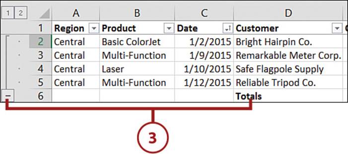
3. Click the last number in the set (in this case, 3) to view the data.
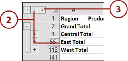
4. Click a + icon to expand a grouping.
5. Click a – icon to collapse a grouping.
Remove Subtotals or Groups
You can remove all the subtotals and groups or choose to remove only outline buttons, leaving the subtotals in place.
1. Select a cell in the grouped data.
2. On the Data tab, click Subtotal.
3. Click Remove All to remove all the subtotals and groups.
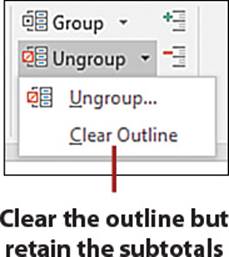
Clear Outline But Retain Subtotals
On the Data tab, click the Ungroup drop-down and then click Clear Outline to remove only the group and outline buttons, leaving the subtotal rows intact.
Toggling the Outline Buttons
Press Ctrl+8 to toggle the visibility of the outline buttons.
Undoing Clear Outline
You cannot undo Clear Outline. If you accidentally select the option, click a cell in the table, bring up the Subtotal dialog box, and click OK. The symbols will be replaced.
Sort Subtotals
If you try to sort a subtotaled dataset while viewing all the data, Excel informs you that to do so will remove all the subtotals. You have to sort each grouped dataset individually.
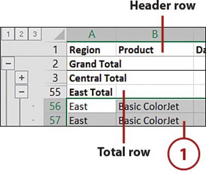
1. Select the cells you want to sort, ensuring no column headers or total rows are included in the range.
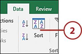
2. On the Data tab, click Sort.
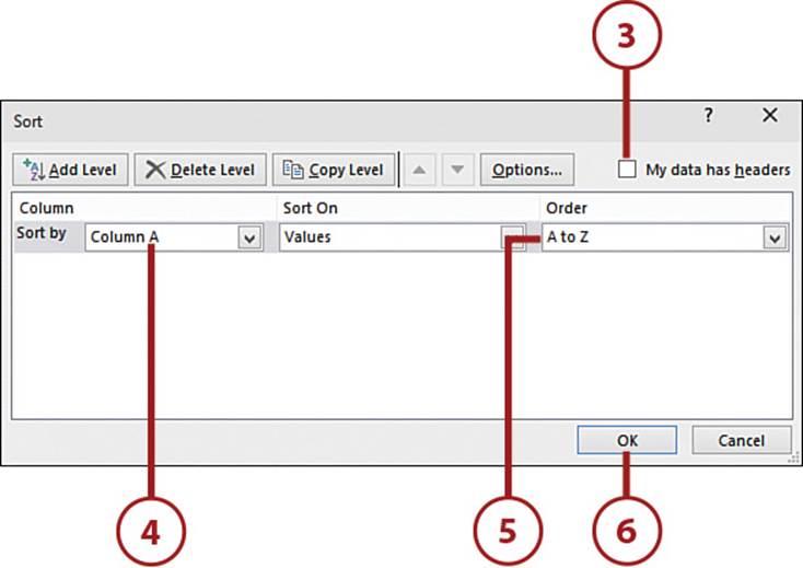
3. Unselect the My Data Has Headers box.
4. Select the column by which to sort.
5. Select the sort order.
6. Click OK. The selected data will be sorted.
Sort Total Rows Only
If you just want to sort the total rows, not the data itself, collapse the dataset so you only see the totals, select a cell in the column with the Total text, and then apply the desired sort.
It’s Not All Good: The Sort Dialog Box Option Changes Stick
If you follow instructions for sorting a dataset and then try to sort the subtotals, you may find your data all messed up. That’s because the changes made in the Sort dialog box, specifically unchecking the My Data Has Headers box, are still in effect. If you are in doubt of what sort settings are in effect, open the Sort dialog box and check.
Copying the Subtotals to a New Location
With a few clicks of the mouse, you can copy and paste just the subtotals to a new location.
Copy Subtotals
Instead of providing all the individual records used to calculate the subtotals, copy and paste just the calculated totals.
1. Click the Outline icon so that only the rows you want to copy are visible.
2. Select the entire dataset. If the headers are to be included, this can be quickly done by selecting a single cell in the dataset and pressing Ctrl+A.
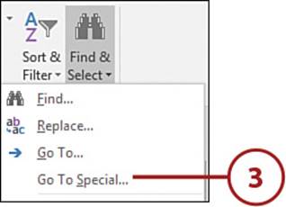
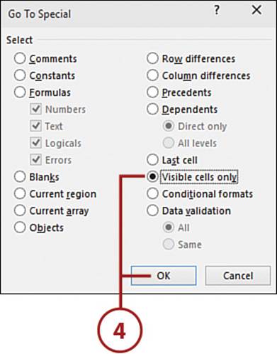
3. On the Home tab, click Go To Special from the Find & Select drop-down.
4. Select Visible Cells Only, and then click OK.
Select Visible Cells Keyboard Shortcut
Instead of using the Go To Special dialog box, press Alt+; (semicolon) to select only the visible cells.
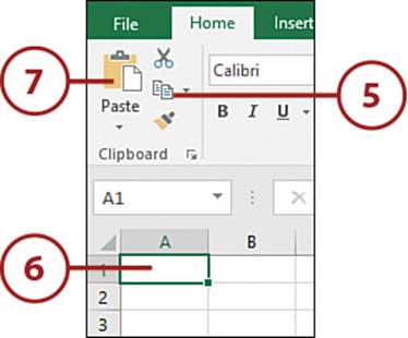
5. On the Home tab, click Copy.
6. Select the top-left cell where the data is to be pasted.
7. On the Home tab, click the Paste button.
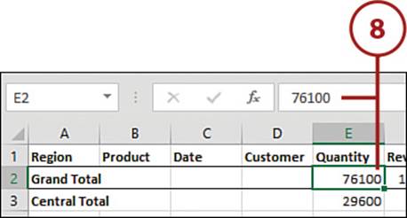
8. The selection is pasted to the new location, and the SUBTOTAL formulas are converted into values.
Formatting the Subtotals
Use steps 1–4 to select the dataset; then, instead of copying the data, apply the desired formatting.
Applying Different Subtotal Function Types
A dataset can have more than one type of subtotal applied to it—for example, a sum subtotal of one column and a count subtotal of another. Because you can only select one function at a time, you will have to use the Subtotal dialog box multiple times.
Create Multiple Subtotal Results on Multiple Rows
You can calculate multiple subtotals to a dataset by using the Subtotal dialog box for each calculation type.
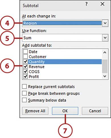
1. Sort the data by the column on which the summary should be based.
2. Select a cell in the dataset.
3. On the Data tab, click Subtotal.
4. Select the column by which to summarize the data—the same column you sorted the data by in step 1.
5. Select the function by which the subtotals should be calculated.
6. Select the column(s) to which the subtotals should be added.
7. Click OK.
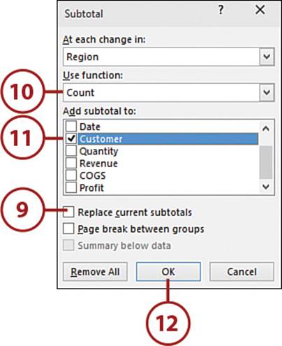
8. On the Data tab, click Subtotal.
9. Uncheck the Replace Current Subtotals box.
10. Select the function by which the subtotals should be calculated.
11. Select the column(s) to which the subtotals should be added.
12. Click OK.
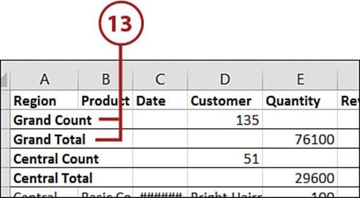
13. The dataset reflects two subtotals, each on its own row.
Combine Multiple Subtotal Results to One Row
When you’re applying multiple function types, Excel places each subtotal on its own row. There is no built-in option to have the subtotals appear on the same row. However, you can manipulate Excel to make this happen by including all the desired columns when setting up the first subtotal. Then, you manually change the formulas to use the subtotal code actually needed.
1. Sort the data by the column on which the summary should be based.
2. Select a cell in the dataset.
3. On the Data tab, click Subtotal.
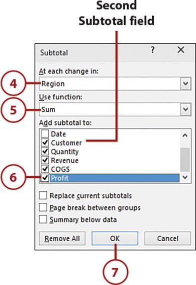
4. Select the column by which to summarize the data—the same column you sorted the data by in step 1.
5. Select the function by which most of the subtotals will be calculated.
6. Select the column(s) to which the subtotals should be added. Include the column to which the second subtotal function would apply. For example, if you’re first applying a sum to Revenue and then applying a count to Customer, include the Customer column now.
7. Click OK.
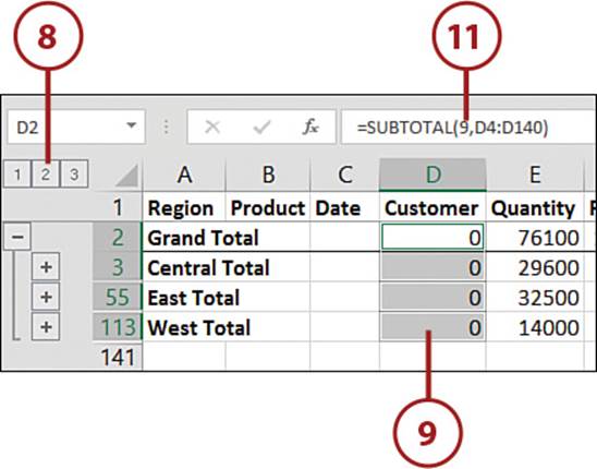
8. Click the “2” icon to collapse the dataset to show only the total rows.
9. Select the data in the column where the second function type should be.
10. Press Alt+; (semicolon) to select the visible cells.
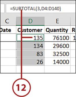
11. In the formula bar, change the current subtotal code to the one you want. For example, to get a count instead of a sum, change the 9 to a 3. Press Ctrl+Enter to apply the change to the selected range.
12. The dataset reflects different types of subtotals on the same row.
Adding Space Between Subtotaled Groups
When subtotals are inserted into a dataset, only subtotal rows are added between the groups. You have two ways to insert extra space into a subtotaled report.
Separate Subtotaled Groups for Print
If the report is going to be printed, blank rows probably don’t need to be inserted. Just the illusion needs to be created because the actual need is for more space between the subtotal and the next group.
1. Collapse the dataset so that only the subtotals are in view.
2. Select the entire dataset, except for the header row.
3. Press Alt+; (semicolon) to select the visible cells only.
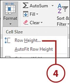
4. On the Home tab, from the Format drop-down, select Row Height.
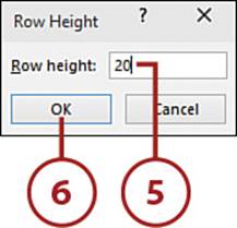
5. Enter a new value in the Row Height dialog box.
6. Click OK.
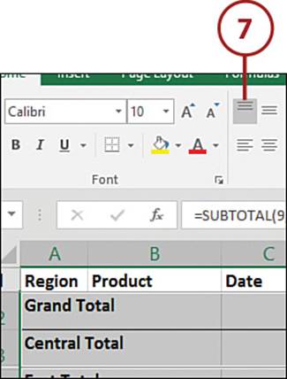
7. If the subtotal rows are below the data, then on the Home tab, select the Top Align button.
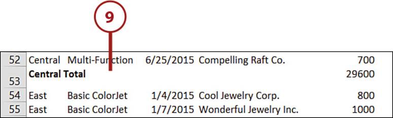
8. Expand the dataset.
9. Spacing now appears between each group.
Separate Subtotaled Groups for Distributed Files
Although the method is a bit involved, a blank row can be inserted between groups in a file that you’re going to distribute. The method involves using a temporary column to mark the space below where a blank row is needed.
It’s Not All Good: Outline Icons Will No Longer Work
This method will disable Excel’s capability to manipulate the subtotals in the dataset. The Total rows will remain, but the outline icons no longer work properly, and future subtotal changes will require the groupings and subtotals to be manually removed first.
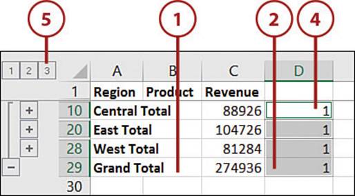
1. Collapse the dataset so only the subtotals are in view.
2. In a blank column to the right of the dataset, select a range as long as the dataset.
3. Press Alt+; (semicolon) to select the visible cells only.
4. Type 1 and press Ctrl+Enter to enter the value in all visible cells.
5. Expand the dataset by clicking the outline icon with the largest number.
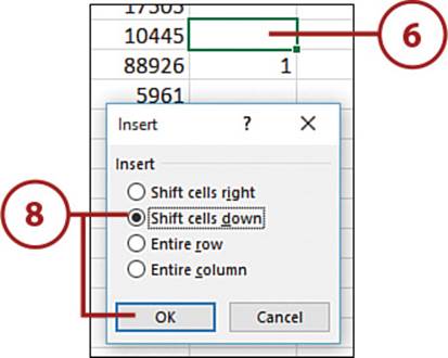
6. Select the cell above the first cell with a 1 in it.
7. On the Home tab, from the Insert drop-down, select Insert Cells.
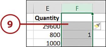
8. Select Shift Cells Down and then click OK. This shifts all the 1’s one row down.
9. Select the column with the 1’s in it.
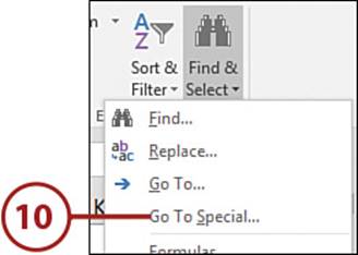
10. On the Home tab, from the Find & Select drop-down, select Go To Special.
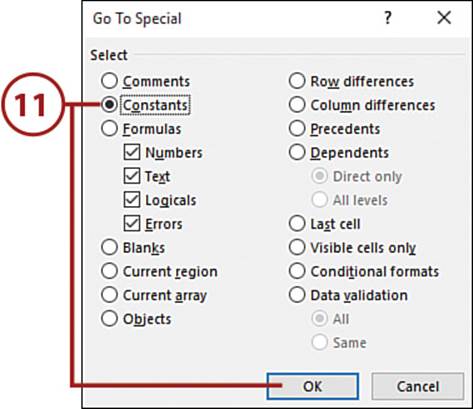
11. From the Go To Special dialog box, select Constants and click OK. Only the 1s are selected.
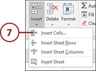
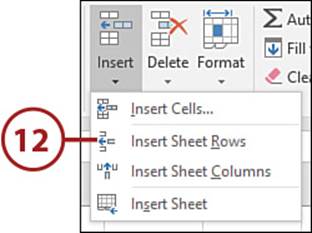
12. On the Home tab, from the Insert drop-down, select Insert Sheet Rows.
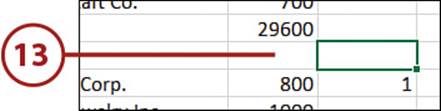
13. A blank row is inserted above each row containing a 1.
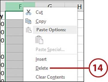
14. Right-click over the temporary column and select Delete.
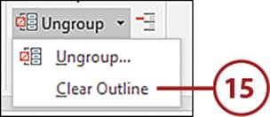
15. Select a cell in the dataset. Then, on the Data tab, from the Ungroup drop-down, select Clear Outline to get rid of the outline icons.
Grouping and Outlining Rows and Columns
You can manually group rows and columns together with or without subtotals. Once the data is grouped, an Expand/Collapse button will be placed below the last row in the selection or to the right of the last column in the selection. An outline can only have up to eight levels.
Selected rows and columns can be grouped together manually using the options in Data, Outline, Group. This is helpful if you have a sheet designed for multiple users and you want to only show rows and/or columns specific to them.
Apply Auto Outline
If the data to be grouped includes a calculated Total row or column between the groups, you can use the Auto Outline option found in the Group drop-down. This option creates groups based on whether the formulas calculate rows or columns. If there are both types of formulas, you’ll get both types of groupings.
1. Select a cell in the dataset.
2. On the Data tab, from the Group drop-down, select Auto Outline.
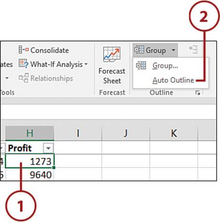
3. The data will be grouped, placing the outline icon on the row or column used to estimate the group.
Group Data Manually
Use the Group option for absolute control over how the rows or columns are grouped.
1. Select a cell in the dataset.
2. On the Data tab, click Subtotal.
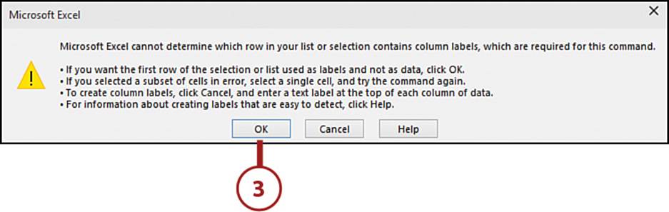
3. A message may appear that Excel cannot determine which row has column labels. Click OK.
4. If you want the outline icons above the data rows they control, ensure Summary Below Data is unchecked. Click OK.
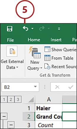
5. Excel inserts subtotal rows in the data. Click the Undo button to remove the rows. Although it may appear that you’ve just undone all the previous steps, these steps are required to configure where the outline icon will appear.
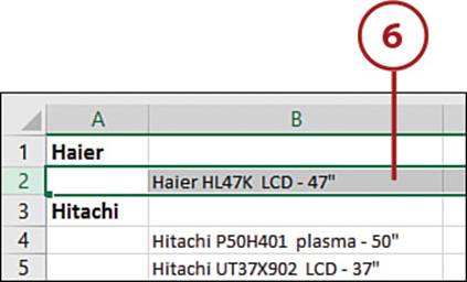
6. Select the first set of rows to group together. Do not include the set’s header. If you have just one row, then select just the one row.
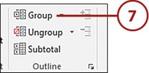
7. On the Data tab, click the Group button.
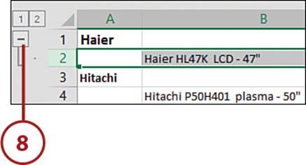
8. The data will be grouped, with an outline icon appearing across from the header.
9. Select the next group of rows and press F4. As long as you don’t perform another command, pressing F4 will repeat the previous action, grouping the selected rows.
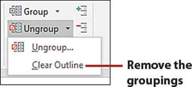
Remove the Groupings
To undo all the groupings, select one cell in the group and then from the Ungroup drop-down, select Clear Outline.
All materials on the site are licensed Creative Commons Attribution-Sharealike 3.0 Unported CC BY-SA 3.0 & GNU Free Documentation License (GFDL)
If you are the copyright holder of any material contained on our site and intend to remove it, please contact our site administrator for approval.
© 2016-2026 All site design rights belong to S.Y.A.