My Excel 2016 (2016)
4. Getting Data onto a Sheet
You never know where your data is going to come from—manually typed in, imported or copied from another file, or from the Web. Because of this, Excel offers a multitude of ways to enter data. In this chapter, you’ll learn those ways and also the following:
→ Entering different types of data
→ Quickly copying data using the fill handle
→ Working with lists
→ Using Text to Columns
→ Controlling user entry with Data Validation
→ Spell checking a sheet
→ Finding data on a sheet
→ Fixing numbers stored as text
Data entry is one of the most important functions in Excel—and one of the most tedious, especially when the data is repetitive. This chapter includes tricks for copying down data, fixing entered data, and helping your users enter data correctly by providing a predefined list of entries.
Entering Different Types of Data into a Cell
Excel treats different types of data, such as numbers and dates, differently. You tell Excel what kind of data is in a cell by how you type it into the cell or by how you format the cell. You can save yourself some time if you let Excel format your data, but it will only do so properly if it can understand what you want.
Type Numbers or Text into a Cell
If you’re entering numbers or text into a cell, just select the cell and start typing.
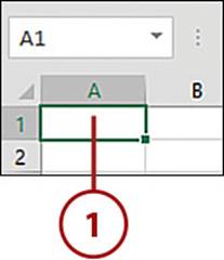
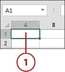
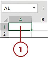
1. Select the cell you want to enter the data into, such as A1.
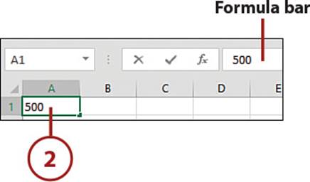
2. Type a value, such as 500. The data will appear in the cell and in the formula bar.
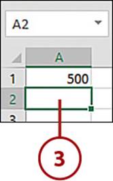
3. Press Enter or Tab to tell Excel you’re done. The active cell will move to the next cell.
Enter Numbers as Text
Suppose you select a cell and type the ZIP code for Chester, MA, which is 01011, and then press Enter or Tab. The beginning 0 disappears, and all you see is 1011. This happens because Excel assumes you are typing in a number, and numbers do not start with zeros. Although ZIP codes are numeric, they aren’t numbers—that is, you don’t do any math with them. You can type an apostrophe to let Excel know the number should be treated as text. The apostrophe does not display.
1. Select the cell you want to enter the data into, such as A1.
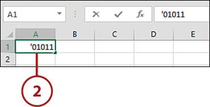
2. Type an apostrophe, and then type the value.
Show That Apostrophe
If you need an apostrophe shown at the beginning of a cell, then enter two apostrophes—only the second one will show when you’re done.
3. Press Enter or Tab to tell Excel you’re done. The active cell will move to the next cell.
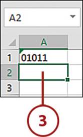
What’s That Green Triangle For?
You’ll notice a small green triangle in the upper-left corner of the cell. This is an Error Checking option. See the section “Fixing Numbers Stored as Text” for more information.
Type Dates and Times into a Cell
Excel uses the system-configured date format by default. For example, in the United States, when you enter numeric dates, the month comes first—that is, May 14, 2015 is written as 5/14/15.
Excel is smart about date and time entry, and if you simply type in dates and times, it does a good job of deciphering your data. When entering times, you must use the 24-hour clock format, also known as military time, or include a.m. or p.m.
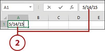
1. Select the cell you want to enter the date into, such as A1.
2. Type a date, such as 5/14/15. The data will appear in the cell and in the formula bar.
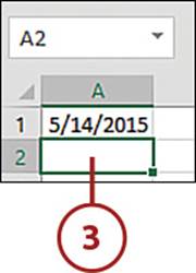
3. Press Enter or Tab to tell Excel you’re done. The active cell will move to the next cell.
For Every Date, There’ a Time
When entering a date, the time (12:00 a.m.) is included. But you might not see the part you didn’t type in until the cell is formatted to show it.
It’s Not All Good: When Fractions Turn into Dates
If you enter only two parts of a date, such as the month and day, Excel will append the current year. But this also means that if you enter a fraction that could be interpreted as date, such as 3/4, Excel will convert it to a date (for example, 3/4/15). To enter a fraction, you must format the cell as Fraction before entering it.
Dates must always include a day, month, and year, even if not all three will appear when the cell is formatted.
See Chapter 6, “Formatting Sheets and Cells,” for more details on applying different number formats and how formatting affects what you see, but not actually what’s in the cell.
Undo an Entry
If you make a mistake, such as in formatting, data entry, or chart creation, you can undo it by click the Undo button. Located in the QAT, the Undo button will undo the most recent action each time it is clicked. If you decide you don’t want to undo an action, you can click the Redo button, which will redo the most recently undone action.

Use Keyboard Shortcuts
Press Ctrl + Z to undo the previous action; press Ctrl + Y to redo the recently undone action.
Using Lists to Quickly Fill a Range
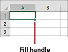
The fill handle can speed up data entry by completing a list for you. Excel comes with several preconfigured lists. You can also add your own list, as described in the “Create Your Own List” section later in this chapter.
Extend a Series Containing Text
Excel comes with custom lists of days of the week and months of the year.
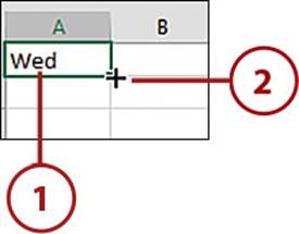
1. Enter the weekday or month you want the list to begin with. Press Ctrl+Enter so Excel accepts the entry, but keeps the cell selected.
2. Place your pointer over the fill handle until a black cross appears.
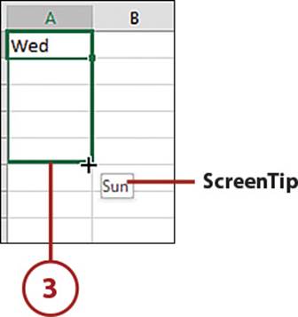
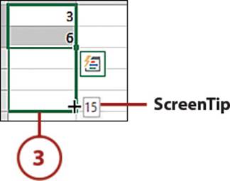
3. Hold the mouse button down as you drag the fill handle. A ScreenTip will show you the value that will be in the cell as you pass it by.
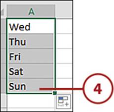
4. Release the mouse button when you’re done making your list.
The List Will Repeat
If you drag the list for more rows or columns than there are values in the list, the list will repeat. For example, if you begin a series in A1 with Wednesday and drag the fill handle to A8, Wednesday will appear again, repeating the series.
Extending Numbers Mixed with Text
If the text series contains a numerical value, Excel copies the text and extends the numerical portion. For example, if you try to extend Monday 1, you get Monday 2, not Tuesday 2. But if you type in Jan 1 and extend that text, Excel extends the numerical portion until Jan 31, then switches to Feb 1. It does this because dates are actually numbers. Seeing the date as Jan 1 is a matter of formatting.
Extend a Numerical Series
If you try to fill numerical series based off of a single cell entry, Excel just copies the value instead of filling the series. Use the following method to get around this:
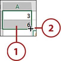
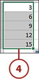
1. Enter and select at least the first two values of the series.
2. Place your pointer over the fill handle so that a black cross appears.
3. Hold the mouse button down as you drag the fill handle. A ScreenTip will show you the value that will appear in the cell as you pass it by.
4. Release the mouse button when you’re done making your list.
>>>Go Further: Alternative Methods
There are a few alternative methods you can choose from to extend a series:
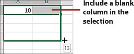
• Enter the first value and hold down the Ctrl key while dragging the fill handle.
• If there is a blank column to the left or right of the numerical column, include that column in your selection when dragging the fill handle down.
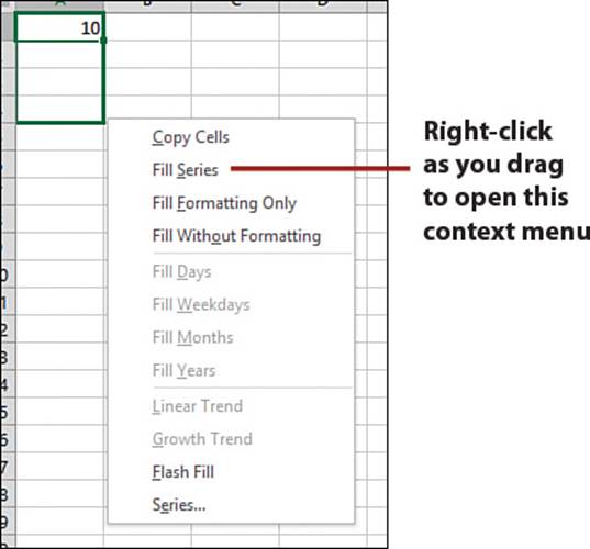
• Hold the right mouse button down while dragging the fill handle and select Fill Series from the context menu that appears when you release the mouse button. This will also work on a series containing text.
Create Your Own List
You can teach Excel the lists that are important to you so that you can take advantage of its list capabilities. You can take almost any list of items on a sheet and create a custom list for use in filtering or sorting.
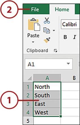
1. Create your list on the sheet and select the range.
2. Click File to enter Backstage view.
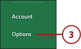
3. Select Options.
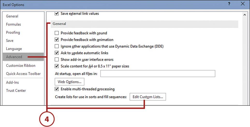
4. Select Advanced, scroll down to General, and click Edit Custom Lists.
5. If your range is not showing in the Import List from Cells field, click the range selector button. Otherwise, skip to step 8.
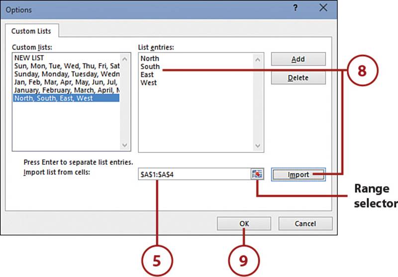
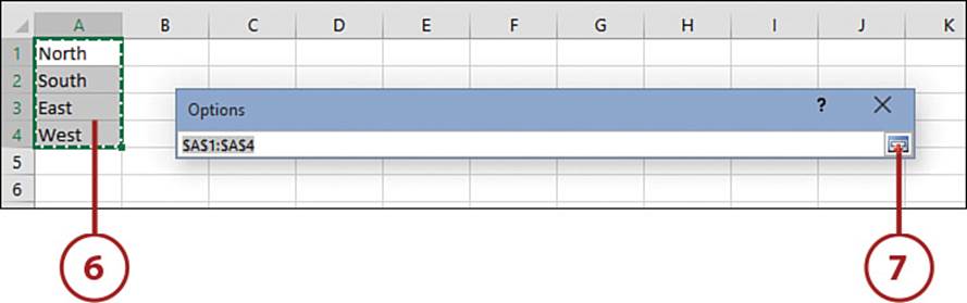
6. Select the list on the sheet.
7. Click the range selector button to return to the dialog box.
8. Click Import. The list is added to both the Custom Lists and List Entries list boxes and will be available for creating custom lists or doing a custom sort or filter.
9. Click OK.
Using Paste Special
The Paste Special dialog box gives you control over how a range is pasted. For example, you can paste values only, formatting only, or a combination of the two. You can also use Paste Special to change the numeric value of a cell.
Paste Values Only
The Values option of the Paste Special dialog box allows you to copy a range containing formulas and paste just the calculated values, replacing the formulas. You can also paste the values to a new location, leaving the original formatting behind.
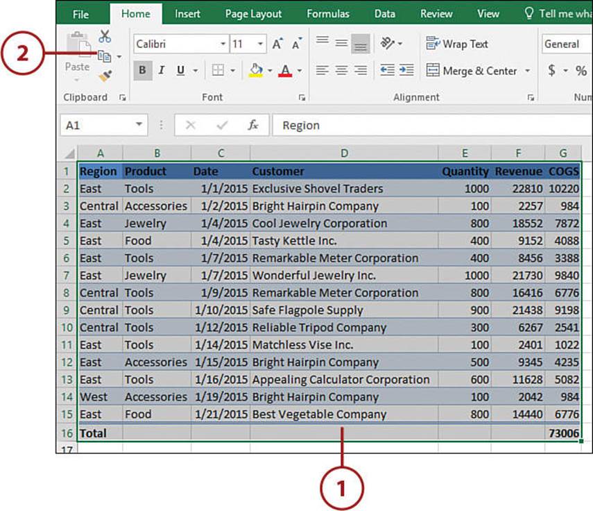
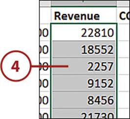
1. Select the range to copy.
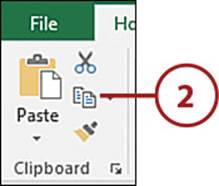
2. On the Home tab, click Copy.
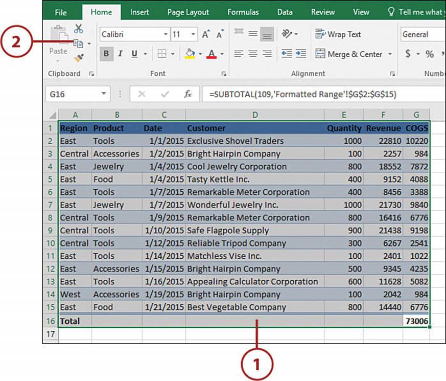
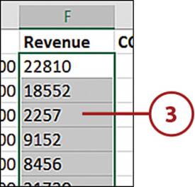
3. Select the top-left cell of the area into which you want to paste.
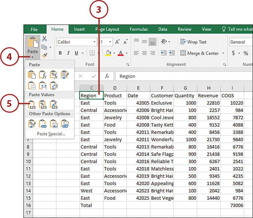
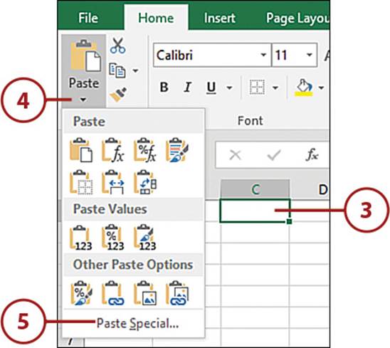
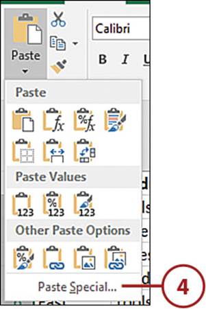
4. On the Home tab, open the Paste drop-down.
5. Select the Values option. The range will be pasted without any of the original formatting.
Paste Preview
You can preview what your pasted range will look like as you move your cursor over the Paste Special options. When you find the one you want, click it.
Combine Multiple Paste Special Options
The Paste drop-down has many different options, but sometimes you may need a combination of data and formatting that isn’t available in the drop-down. The Paste Special dialog box allows you to choose individual properties of the copied range that you want pasted, and by using the dialog box multiple times in succession, you can stack the properties. For example, you might want to paste values and also retain the column widths. In that case, use the Paste Special dialog box twice in succession, as described in the following steps.
1. Select the range to copy.
2. On the Home tab, click Copy.
3. Select the top-left cell of the area into which you want to paste.
4. On the Home tab, open the Paste drop-down.
5. Select the Paste Special option.
6. Select Values.
7. Click OK.
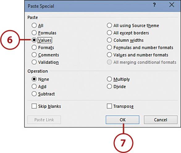
8. Only the values will be pasted into the cells.
9. Reopen the dialog box and select Column Widths.
10. Click OK.
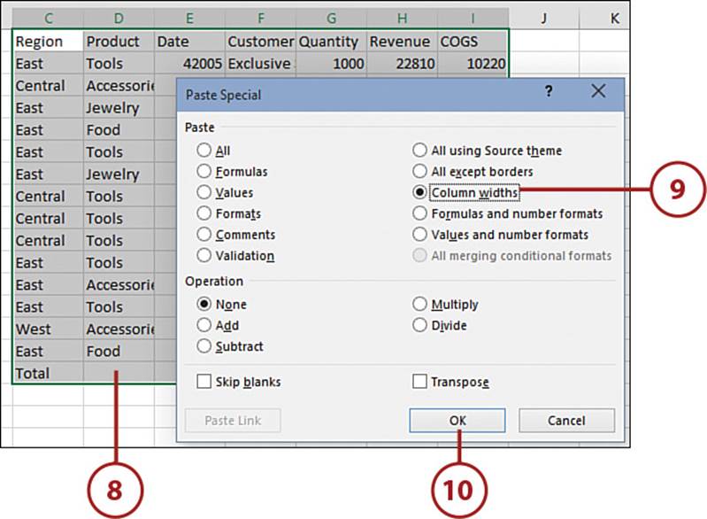
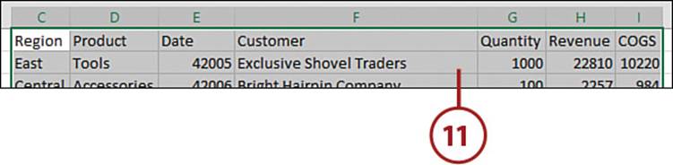
11. The column widths used by the copied range will be duplicated onto the pasted range.
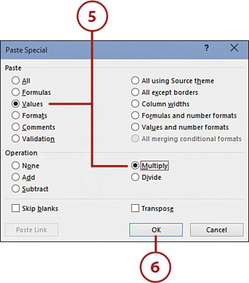
Multiply the Range by a Specific Value
The Operation area in the Paste Special dialog box allows you to perform simple math on a selected range, such as increasing all prices by 15%.
1. In any blank cell on the sheet, enter the value by which you want to change the range. For example, to increase by 15%, enter 1.15.
2. Copy the cell by clicking the Copy button on the Home tab.
3. Select the range you want to update.
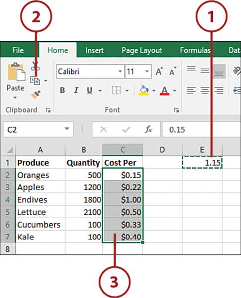
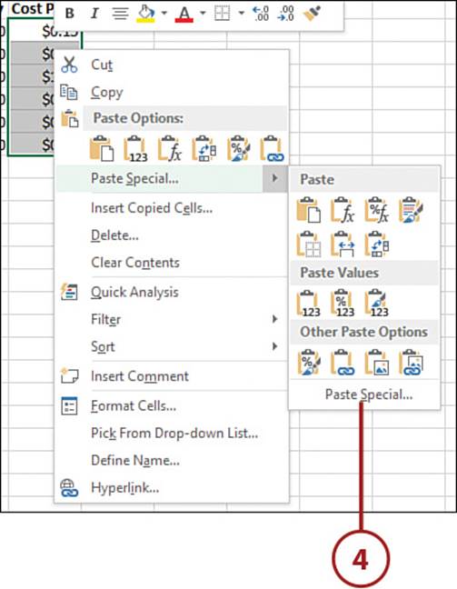
4. Right-click over the selected range and select Paste Special, Paste Special.
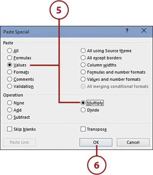
5. Select Values, so you don’t replace the formatting of the range, and then select Multiply, the mathematical operation you want to perform on the range.
6. Click OK.
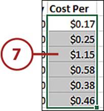
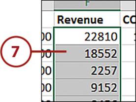
7. Excel will update the values in the selected range.
>>>Go Further: Paste Special with Non-Range or Non-Excel Sources
If you copy or cut data within a cell (versus the entire cell), from a chart, or from a non-Excel source, such as a Word document or web page, the Paste Special options are limited, depending on the original source.
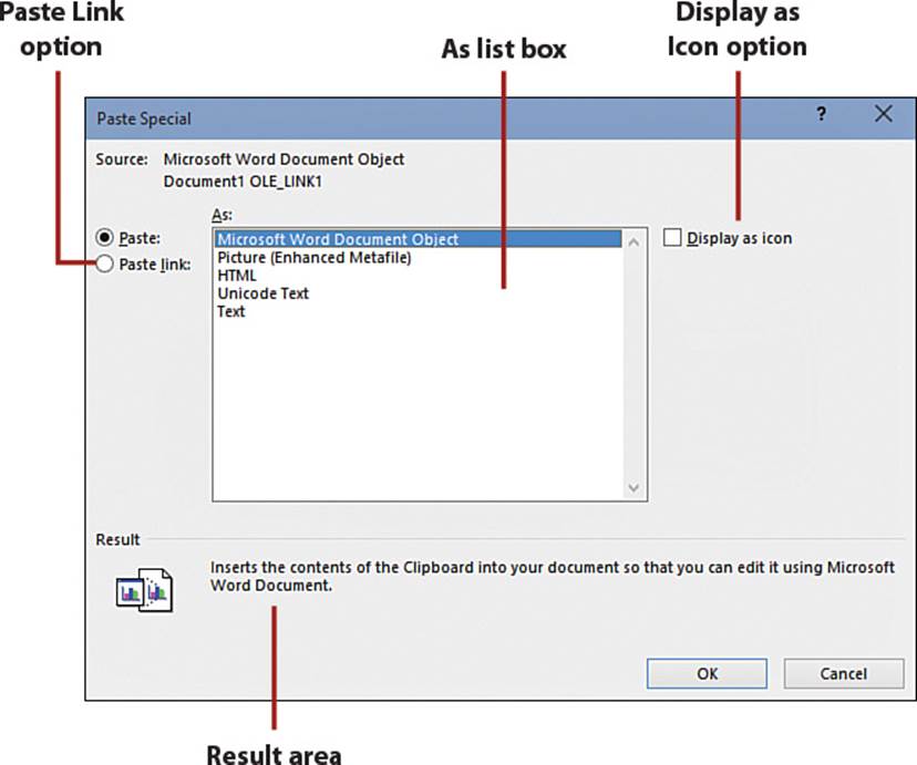
As you select an option in the As list box, an explanation appears in the Result area at the bottom of the dialog box. Selecting the Paste Link option also links the pasted data to its original source.
If available, the Display as Icon option lets you paste an icon instead of the text. Double-clicking the resulting icon in the worksheet opens the text in an editing application. (For example, if you’re pasting text from a Word document, you can edit the text in Word.)
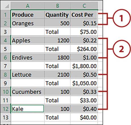
Use Paste to Merge a Noncontiguous Selection
If you try to copy/paste a noncontiguous selection from different rows and columns, an error message appears. But if the selection is in the same row or column, Excel allows you to copy and paste the data. When the data is pasted, though, it is no longer separated by other cells. You can use this method to create a range of specific values copied from another dataset.
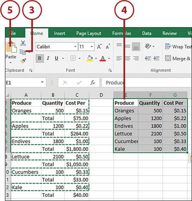
1. Select the first range you want to copy.
2. While holding down the Ctrl key, select the other ranges.
3. On the Home tab, select Copy.
4. Select the top-left cell where you want the new range to go.
5. On the Home tab, select Paste. The data will be pasted together.
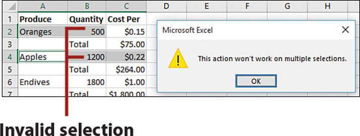
This Action Won’t Work on Multiple Selections
For Excel to see the selection as a single selection, it must be stacked—that is, it must start and end in the same columns or rows.
Using Text to Columns to Separate Data in a Single Column
Importing data from other sources, such as databases, is a common use of Excel. Often, the files generated by these other sources are delimited by a common character, such as a comma, or are fixed width, where each field is a specific number of characters, including spaces.
If you open a file like this in Excel, you can use Text to Columns to parse the data out from one column into individual columns for each field.
Parsing a Column in the Middle of an Existing Dataset
If you need to parse a column in the middle of an existing dataset, you first need to insert enough columns to cover the number of columns the parsed data will use. Otherwise, it will overwrite any data to the right of the original column.
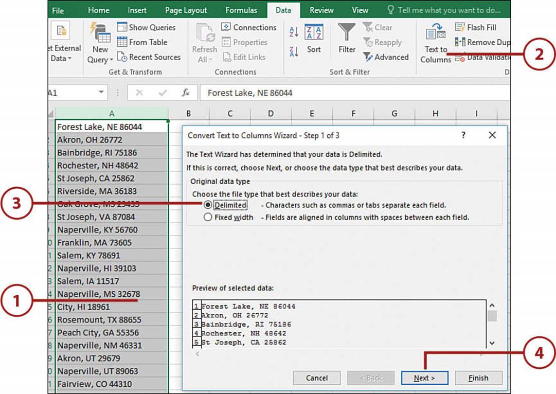
Work with Delimited Text
Delimited text is data that has some character, such as a comma, tab, or space, separating each value that you want placed into its own column.
1. Highlight the range to be separated.
2. On the Data tab, select Text to Columns. The Convert Text to Columns Wizard opens.
3. Select Delimited.
4. Click Next.
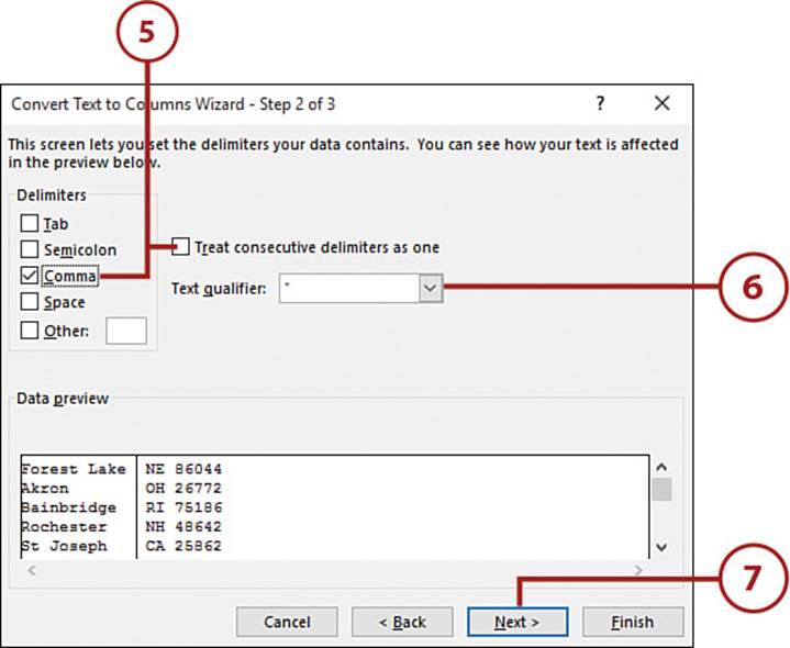
5. Select the delimiter or enter one in the Other field. If multiple delimiters may be next to each other but should be treated as one, select Treat Consecutive Delimiters as One.
6. If you have quotation marks or apostrophes around the text fields in the data, select the corresponding Text Qualifier.
7. Click Next.
Multiple Delimiters
If you need more than one delimiter but one of the delimiters is used normally in the text, such as the space between city names and the space between a state and ZIP code (Sioux Falls, SD 57101), consider running Text to Columns twice: once to separate the city (Sioux Falls) from the state ZIP code (SD 57101) and again to separate the state and ZIP code.
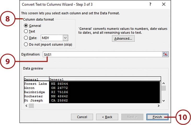
8. For each column of data, click on the column’s header then select the data format for that column. For example, if you have a column of ZIP codes, you need to set the format as Text so any leading zeros are not lost. But be warned—setting a column to Text prevents Excel from properly identifying formulas entered into that column.
9. If you want the results placed in a different location, place your cursor in the Destination field and then select a new target cell.
10. Click Finish.
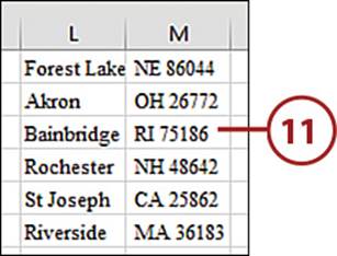
11. The data is separated.
>>>Go Further: Work with Fixed-Width Text
Text to columns also works with fixed-width text, which is text where each field is a set number of characters. If your text doesn’t look like it’s a fixed width, try changing the font to a fixed-width font, such as Courier. It’s possible that it’s fixed-width text in disguise.
When you select this option, instead of choosing a delimiter, Excel shows a preview with lines where it thinks the column breaks should go. You can move a break line by clicking and dragging it to where you want it. You can insert a new break by clicking where it should be, and you can remove a break by double-clicking it.
Using Data Validation to Limit Data Entry in a Cell
Data validation allows you to limit what a user can type in a cell. For example, you can limit users to whole numbers, dates, a list of selections, or a specific range of values. Custom input and error messages can be configured to guide the user entry.
Limit User Entry to a Selection from a List
A data validation list allows you to create a drop-down in a cell, thus restricting the user to selecting from a predefined list of values.
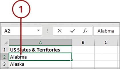
1. Create a list of the values to appear in the drop-down. For example, in A1, type Apples, in A2, Oranges, and so on.
Protect the List By Placing It on Another Sheet
You can place the list on a sheet other than the one where the drop-down will actually be placed. You can then hide that sheet, thus preventing the user from changing the list.
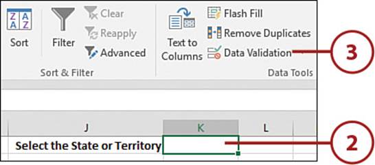
2. Select the cell in which you want the drop-down to appear.
3. On the Data tab, select Data Validation.
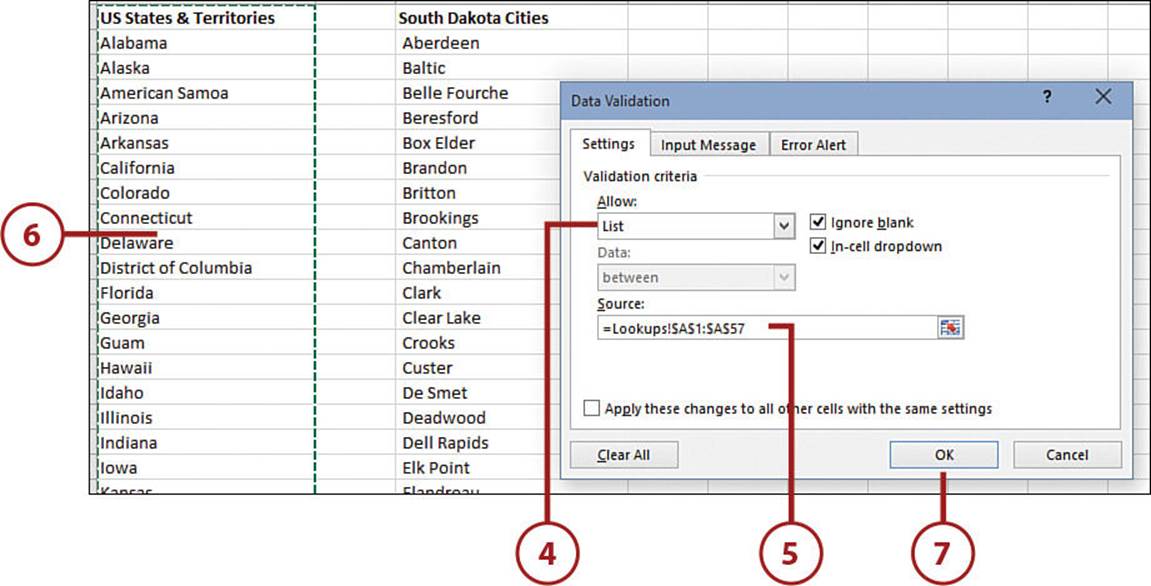
4. Select List from the Allow drop-down.
5. Place your cursor in the Source field.
6. Select the list you created in step 1.
7. Click OK.
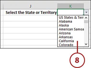
8. The cell selected in step 2 is now a drop-down. Users will be limited to values in the list.
Skip the List
If your list is short, instead of the separate list you created in step 1, you can enter the values separated by commas directly in the Source field. For example, in the Source field you could enter Yes, No (no quotes, no equal sign).
Add a Prompt or Error Message
If you want to provide the user with an input prompt, go to the Input Message tab and fill in the Title and Input Message fields.
If you want to provide the user with an error message, go to the Error Alert tab and fill in the Style, Title, and Error Message fields.
>>>Go Further: Other Validation Options
A drop-down list isn’t the only way to validate data. Other available validation criteria include the following:
• Any Value—The default option allowing unrestricted entry.
• Whole Number—Requires a whole number be entered. You can select a comparison value (Between, Not Between, Equal To, and so on) and set the Minimum and Maximum value.
• Decimal—Requires a decimal value be entered. You can select a comparison value (Between, Not Between, Equal To, and so on) and set the Minimum and Maximum values.
• Date—Requires a date be entered. You can select a comparison value (Between, Not Between, Equal To, and so on) and set the minimum and maximum values.
• Time—Requires a time be entered. You can select a comparison value (Between, Not Between, Equal To, and so on) and set the minimum and maximum values.
• Text Length—Requires a text value be entered. You can select a comparison value (Between, Not Between, Equal To, and so on) and set the minimum and maximum number of characters.
• Custom—Uses a formula to calculate TRUE for valid entries or FALSE for invalid entries.
Using Web Queries to Get Data onto a Sheet
Excel can be used to retrieve data from a website, if the site has been designed in such a way that Excel can find the tables on it. A link is created so the data on the sheet will update as often as you wish.
Insert a Web Query
A web query allows you to link a range to data from a web page. As the web page updates, the data on the sheet also updates.
1. On the Data tab, open the Get External Data drop-down and select From Web.
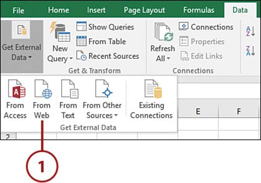
No Get External Data Drop-Down
If your screen resolution is set high enough, you won’t have a Get External Data drop-down. Instead, the From Web button will be directly on the Data tab.
2. In the New Web Query dialog box, navigate to the desired web page.
Script Errors
If you receive Script Errors while loading the web page, click Yes to allow scripts to continue and the page to load.
3. Resize the window if needed by clicking and dragging the lower-right corner.
4. A box with an arrow appears near the data that can be retrieved. Place your pointer over the box, and it changes color. A frame appears around the data that box is tied to.
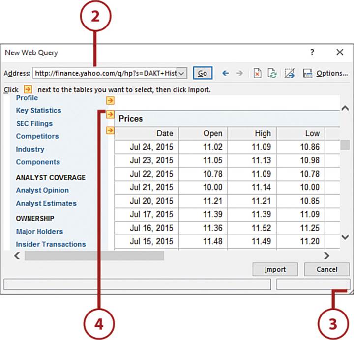
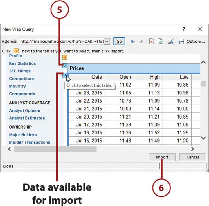
5. Click the box, and it turns into a box with a check mark.
6. Select as many sections as you need; then click Import.
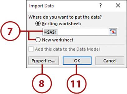
7. Select the cell where you want the data to appear. To change the current cell address shown, click the correct cell. If you want the entry on a new sheet, select the New Worksheet option.
8. Click Properties.
9. Select the Refresh Every check box and enter how often (in minutes) you want the data refreshed.
10. Click OK.
11. Click OK.
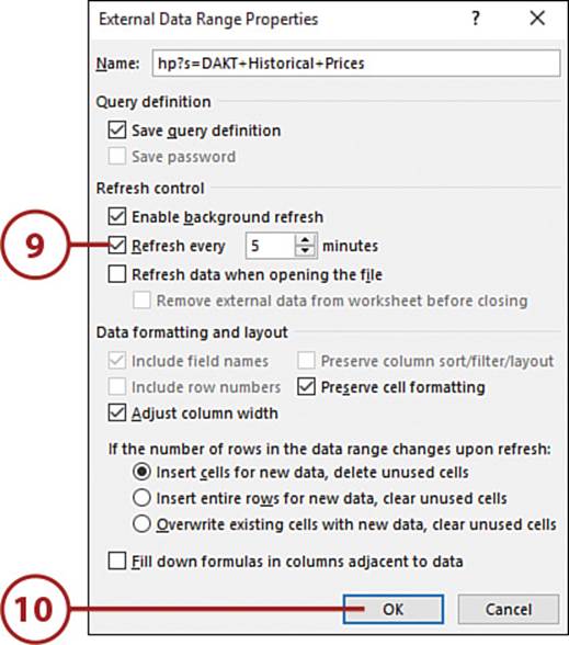
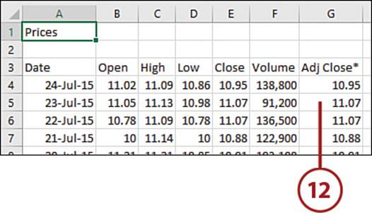
12. After a few seconds, depending on your Internet connection, the data appears on the sheet.
Editing Data
Now that you know how to enter data into a blank cell, how do you edit data already in a cell? If you select a cell and start typing, you’ll overwrite what was originally in the cell.
Modify Cell Data
You can modify the data in a cell without retyping it.
1. Double-click a cell, and the cursor appears in that cell.
Alternative Methods
You can also enter edit mode on a cell by selecting a cell and then clicking where you want to edit in the formula bar. Or, you can select the cell and press F2. The cursor will appear at the right end of the data in the cell.
2. When you’re done making changes, press Tab or Enter to exit out of the cell and save your changes. If you change your mind about the changes while you’re still in the cell, press Esc and you’ll exit the cell without saving your changes.
Clearing the Contents of a Cell
When you delete a cell, you remove it from the sheet and other cells move to take fill the space. If you want to delete only the data, leaving the cell intact, you have to clear it.
Clear Only Data from a Cell
Clear a cell to remove the data but retain the formatting.
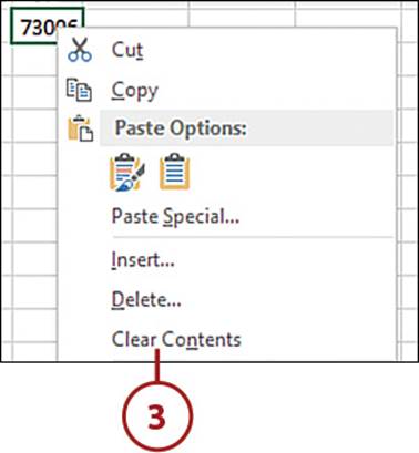
1. Select the cell to clear.
2. Press Delete on the keyboard. The data in the cell is deleted.
Or
3. Right-click over the cell and choose Clear Contents.
Don’t Use the Spacebar!
You may be tempted to use the spacebar to clear a cell. Don’t! Although you can’t see the space in the cell, Excel can. That space can throw off Excel’s functions because to Excel, that space is a character.
Clearing an Entire Sheet
You can clear all data from a sheet without actually deleting the sheet.
Clear an Entire Sheet
You quickly delete all cells from a sheet, or the data only, retaining the formatting.
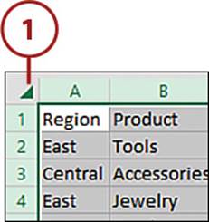
1. Click the intersection between the headings. This will select all the cells on the sheet.
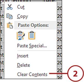
2. To clear a sheet of all data, but leave any formatting intact, press Delete on the keyboard or right-click and choose Clear Contents.
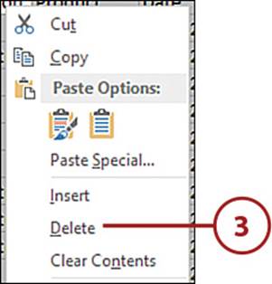
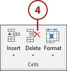
3. To clear a sheet of all data and formatting, right-click and select Delete.
Or
4. On the Home tab, select Delete.
Working with Tables
Excel also has a special format, table, you can apply to a dataset, imbuing it with special abilities and rules. When your dataset is defined as a table, additional functionality in Excel is made available. For example, with Excel’s intelligent tables, the following additional functionality becomes available:
• AutoFilter drop-downs are automatically added to the headers.
• You can apply predesigned formats, such as banded rows or borders.
• You can remove duplicates based on the values in one or more columns.
• You can toggle the Total Row on and off.
• Adding new rows or columns automatically extends the table.
• You can take advantage of automatically created range names.
>>>Go Further: Get the Most out of Tables
This section is a brief introduction to tables. To get the most out of a table, check out Excel Tables: A Complete Guide for Creating, Using, and Automating Lists and Tables by Zack Barresse and Kevin Jones (ISBN: 978-1615470280).
Define a Table
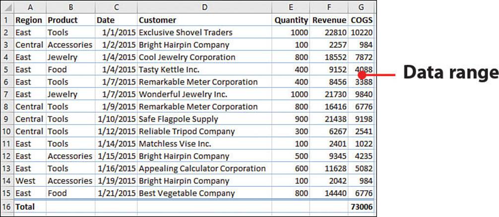
For a dataset to convert to a table, it must be set up properly. This means that, except for the header row, each row must be one complete record of the dataset—for example, a customer or inventory item. Column headers are not required, but if they are included, they must be in the row at the top of the dataset. If your data does not include headers, Excel inserts some for you.
1. Select a cell in the dataset.
2. On the Insert tab, select Table.
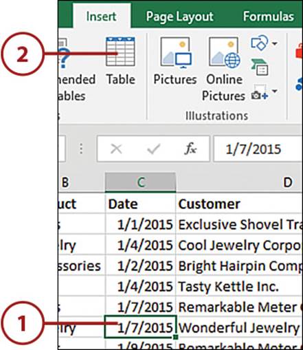
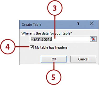
3. Excel will determine the range of the dataset. If what is shown is incorrect, click the sheet and select the dataset.
Excel Doesn’t Select Your Entire Dataset
When Excel is determining what cells belong together in a dataset, it does this by looking for empty rows and columns. If you have any empty rows or columns in the middle of your dataset, Excel will see them as the end of the table.
4. If your dataset has headers, be sure My Table Has Headers is selected.
5. Click OK.
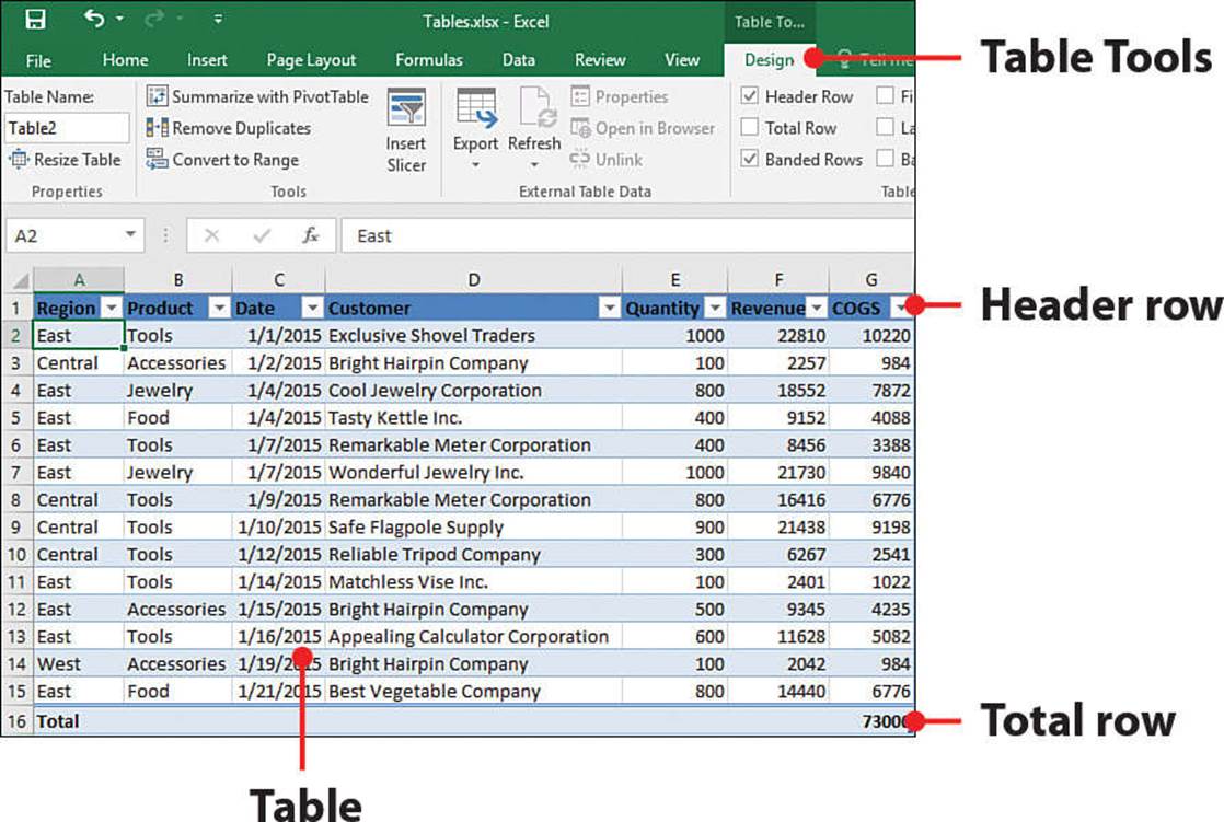
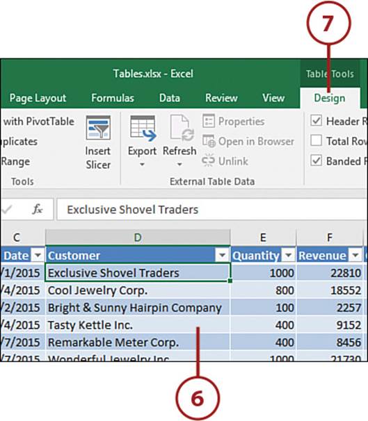
6. Excel converts the dataset to a table and applies the default formatting and settings.
7. A new tab called Table Tools, Design appears in the ribbon. Whenever you select a cell in a table, this tab appears. It contains functionality and options specific to tables.
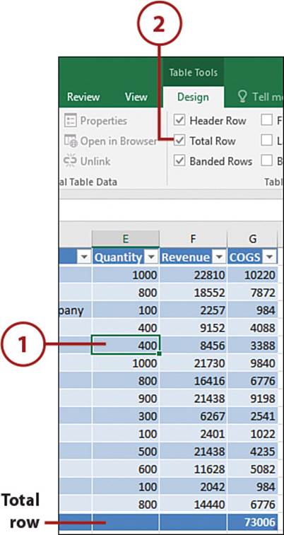
Add a Total Row to a Table
When you add a total row to your table, Excel adds the word Total to the first column of the table and sums the data in the rightmost column. If the rightmost column contains text, Excel returns a count instead of a sum.
1. Select a cell in the table to display the Table Tools ribbon tab.
2. On the Table Tools, Design tab, select Total Row. Excel will add a total row to the bottom of the table.
Change the Total Row Function
Each cell in the total row has a drop-down of functions that can be used to calculate the data above it.
1. Select the cell in the total row that you want add a Total function to.
2. Open the drop-down list.
3. Select the desired function.
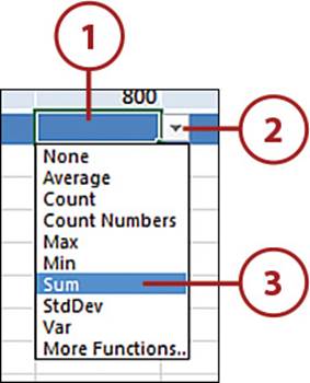
4. Excel will insert the correct formula in the cell.
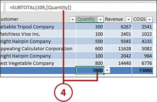
Total Rows Using the SUBTOTAL Function
The functions listed in the drop-down are calculated using variations of the SUBTOTAL function. For more information on this function, see Chapter 13, “Inserting Subtotals and Grouping Data.”
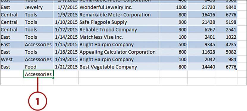
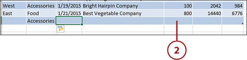
Expand a Table
As you enter text in adjacent rows and columns, the table automatically expands to include them.
1. Enter data in a cell in the next available row and then press Tab or Enter.
Expansion When Entering Multiple Records
The table will also automatically add a new row when you enter a value in the last row and column and then press Tab.
2. The table expands to include the new row.
Stop Automatic Expansion
A table automatically expands as you add adjacent rows and columns. If you don’t want the new entry to be part of the table, you can tell Excel by clicking the lightning bolt icon that appears and then selecting either Undo Table AutoExpansion or Stop Automatically Expanding Tables. If you choose Stop Automatically Expanding Tables, this will stop automatic expansion for future tables as well.
Turn Off the Total Row
When adding new rows to the bottom of a table, make sure the Total row is turned off; otherwise, Excel cannot identify the new row as belonging with the existing data. The exception is if you tab from the last data row, Excel inserts a new row and moves the Total row down.
Fixing Numbers Stored as Text
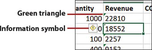
Sometimes when you import data or receive data from another source, the numbers might be converted to text. When you try to sum them, nothing works. That is because Excel will not sum numbers stored as text.
When numbers in a sheet are being stored as text, Excel lets you know by placing a green triangle in the cell. When you select the cell, an information symbol appears. The following two sections show you how to convert these values to true numbers so that calculations can be performed.
No Green Triangle
If you have numbers stored as text but don’t see a green triangle, it’s possible you have the Error Checking feature turned off. To check, and turn it on, go to File, Options, Formulas, Error Checking, Enable Background Error Checking.
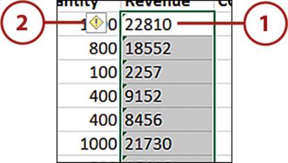
Use Convert to Number on Multiple Cells
One option for converting multiple cells into numbers is to use the Convert to Number option in the information symbol.
1. Select the range you need to convert, making sure that the first cell in the range needs to be converted. The range can include text and other numerical values, as long as it doesn’t include cells you do not want to be converted to numbers.
2. Click the information symbol in the first cell.
3. From the drop-down, select Convert to Number.
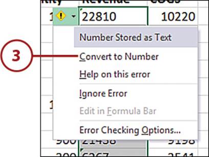
4. All cells in the selected range will be modified, turning the numbers to true numbers. The green triangles will go away.
Use Paste Special to Force a Number
If you have Background Error Checking disabled or don’t see the green warning triangle, try this method for converting cells to numbers.
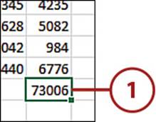
1. Enter a 1 in a blank cell. Press Ctrl+Enter so that Excel accepts the value but the cell also remains the active cell.

2. On the Home tab, select Copy.
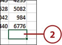
3. Select the cells containing the numbers to convert.
4. On the Home tab, select Paste Special from the Paste Special drop-down.
5. Select the Values and Multiply options.
6. Click OK.
7. All cells in the selected range will be modified, turning the numbers to true numbers.
The act of multiplying the values by 1 forces the contents of the cells to become their numerical values.
Spell Checking a Sheet
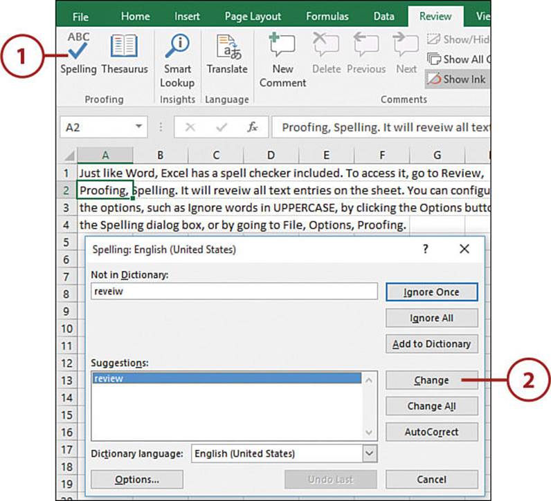
Just like Word, Excel has a spell checker included. It reviews all text entries on the sheet.
1. On the Review tab, select Spelling.
2. As Excel goes through the sheet, select the desired option, such as Change to correct a misspelling.
Finding Data on a Sheet
Through the Find and Replace dialog box, you can find data on any sheet in the workbook.
Perform a Search
When you perform a search, Excel will select the matching cell.
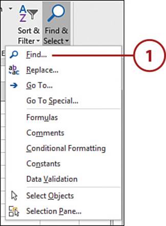
1. On the Home tab, select Find from the Find & Select drop-down.
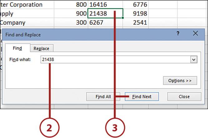
2. Enter your search term.
3. Click Find Next. Excel will select a cell containing the term.
Or
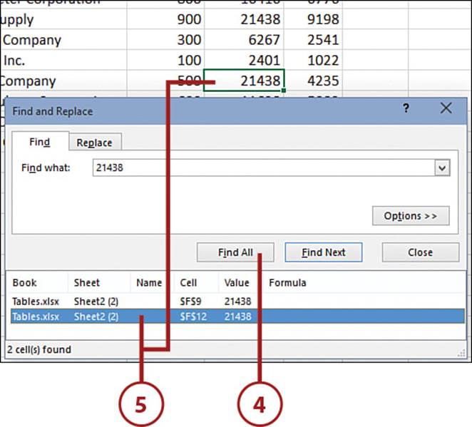
4. Click Find All. Excel will select a cell containing the term and also provide a list of all cells with the term.
5. You can click a row in the search results, and Excel will jump to that selection.
>>>Go Further: Refine Your Search
If you click the Options button on the Find and Replace dialog box, several options appear to help you refine your search:
• Within—You can search just the active sheet or the entire workbook. You can also narrow Excel’s search by selecting the range before bringing up the dialog box.
• Search—To have the search go down all the rows of one column before going on to the next column, set this to By Rows. To have the search go across all columns in a row before going on to the next row, select By Columns.
• Look In—By default, Excel looks in formulas (that is, the true value of the data in a cell). When you’ve applied formulas or formatting to a sheet, what you see in a cell might not be what is actually in the cell. To search for the value, what you see in the cell, change the drop-down to Values. You can also choose to search in comments.
It’s Not All Good: When Find Doesn’t Work
You perform a Find operation for a value (for example, 123) you know is on the sheet, but Excel says it cannot find it. You find the value manually, and it’s actually 123.18, but you know this method worked before—so why not this time?
You look at the options and notice Match Entire Cell Contents is selected. You had selected it earlier in the day when you were searching in another workbook.
The settings in the Find and Replace dialog box are stored throughout an Excel session. This means that if you change them in the morning for a search and then try a different search later in the afternoon without having closed Excel at all during the day, the settings changes you’ve made are still active, even if you’re searching a different workbook.
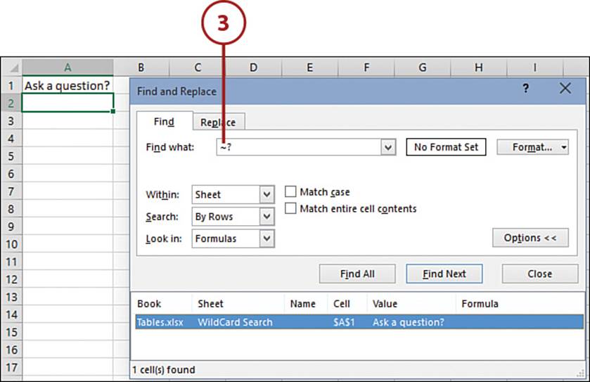
Perform a Wildcard Search
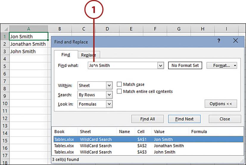
What if you don’t know the exact text you’re looking for? Wildcards can be added to the search term, each wildcard helping in a different way.
1. Use an asterisk (*) in the search term to tell Excel there might or might not be additional characters between two known characters.
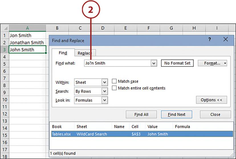
2. Use a question mark (?) to replace an unknown character.
3. If you need to include the * or ? as part of your search term, not as a wildcard, the use the tilde (~) symbol to tell Excel the character is an actual text character. If your search term character is a ~, then you would have two in the search term.
Replace Data on a Sheet
You can replace data as you find it, or replace all matches with a single click.
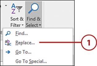
1. On the Home tab, select Replace from the Find & Select drop-down.
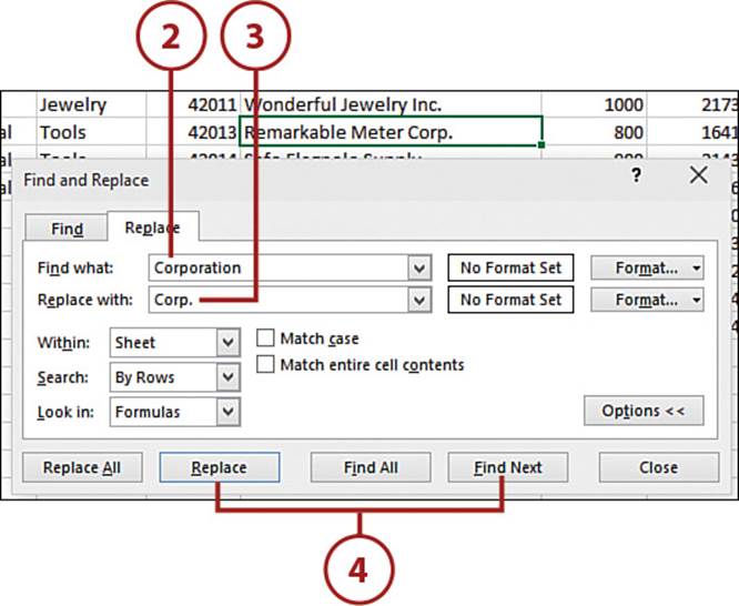
2. Enter your search term.
3. Enter the term you want to replace it with.
4. Click Find Next. Excel will select a cell containing the term. If you want to replace the term in that cell, click Replace. If you don’t want to replace that instance, click Find Next. Repeat this step until all desired replacements are made.
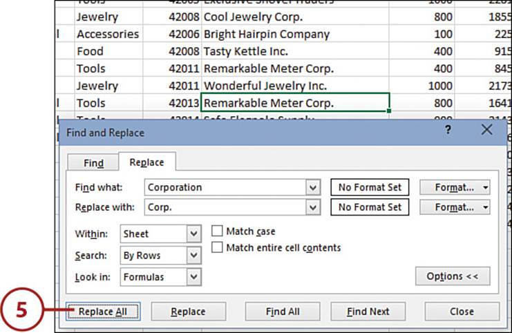
Or
5. Click Replace All. Excel will replace all instances of the term.
Find and Replace Formatting
Through the Format buttons on the Find and Replace dialog box, you can narrow down your search by choosing the formatting the desired matches have, such as the number format or font. You can also use the Format option to apply a format to matches.
All materials on the site are licensed Creative Commons Attribution-Sharealike 3.0 Unported CC BY-SA 3.0 & GNU Free Documentation License (GFDL)
If you are the copyright holder of any material contained on our site and intend to remove it, please contact our site administrator for approval.
© 2016-2026 All site design rights belong to S.Y.A.