My Excel 2016 (2016)
6. Formatting Sheets and Cells
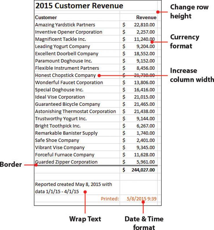
Formatting data is important—it makes it easier to interpret the data and pulls the user’s eye to important parts. You also need to know how to resize rows and columns so more of your data is visible. This chapter includes the following topics:
→ Merging cells
→ Formatting dates
→ Centering data in a cell
→ Quickly copying a format from one range to another
→ Switching between number formats
Now that you have your data on a sheet, you need to format it so that it’s easy to decipher and readers can quickly make sense of it. From formatting the font, wrapping text, and merging cells to changing how a number is displayed in a cell, Excel has the tools you need to make reports visually interesting.
Changing the Font Settings of a Cell
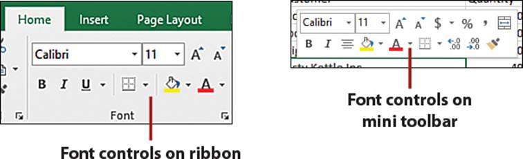
Changing font aspects allows you to add emphasis to an entire cell. Two ways you can access the font-changing tools in Excel are from the ribbon and from the mini toolbar, which is accessed by right-clicking over a range.
>>>Go Further: Change Multiple Font Settings at a Time
The following sections will outline how to change one font setting at a time, but on the Font tab of the Format Cells dialog box, you can change multiple settings at one time.
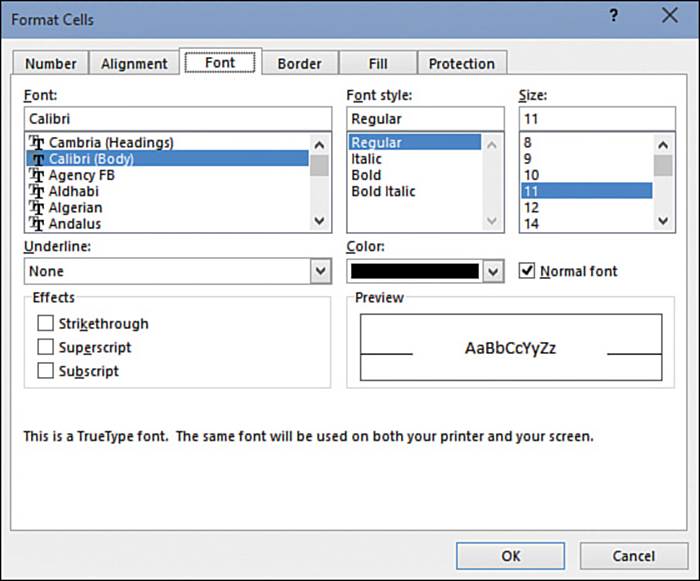
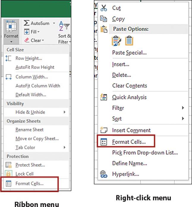
To open the dialog box, select Format Cells from the Format drop-down on the Home tab or right-click over a selected range and choose Format Cells.
Select a New Font Typeface
The default font in Excel is Calibri, but many others are available.
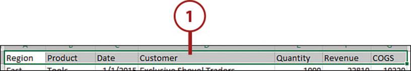
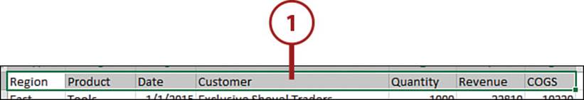
1. Select the range for which you want to change the font.
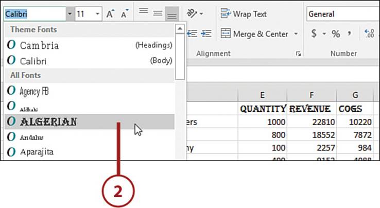
2. On the Home tab, open the Font drop-down and click the desired font.
Use the Mini Toolbar
You can also change the font using the mini toolbar. Right-click over the selected range and click a font from the Font drop-down of the mini toolbar.
Preview Your Selection
If the selected range is in view, you can preview the font change as you move your mouse pointer across fonts on the list. When you find the one you want, click it to make the change stick.
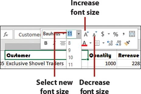
Increase and Decrease the Font Size
The default font size in Excel is 11, but you can make it smaller or larger.
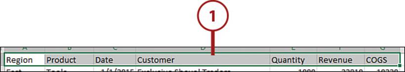
1. Select the range for which you want to change the font size.
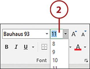
2. On the Home tab, open the Font Size drop-down and click the desired size.
Other Ways to Change the Font Size
You can change the font using the mini toolbar. Right-click over the selected range and select a size from the Font Size drop-down of the mini toolbar.
Both the ribbon and mini toolbar include buttons to increase and decrease the font size. Click the Increase Font Size button and the font will increase to the next size; click the Decrease Font Size button and the font will decrease to the previous size.
Apply Bold, Italic, and Underline to Text
In addition to changing the font type or size to add emphasis to data, you can bold, italicize, or underline the values.
1. Select the range you want to format.
2. On the Home tab, click the desired font style.
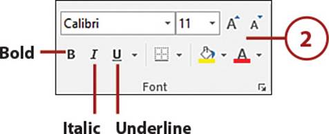
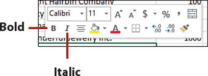
Use the Mini Toolbar
You can bold and italicize the font using the mini toolbar. Right-click over the selected range and select the desired font style on the mini toolbar.
Use Keyboard Shortcuts
The popular keyboard shortcuts for bold (Ctrl+B), italic (Ctrl+I), and underlining (Ctrl+U) also work in Excel.
Apply Strikethrough, Superscript, and Subscript
The strikethrough, superscript, and subscript effects are available only through the Format Cells dialog box.
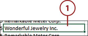
1. Select the range to which you want to apply an effect.
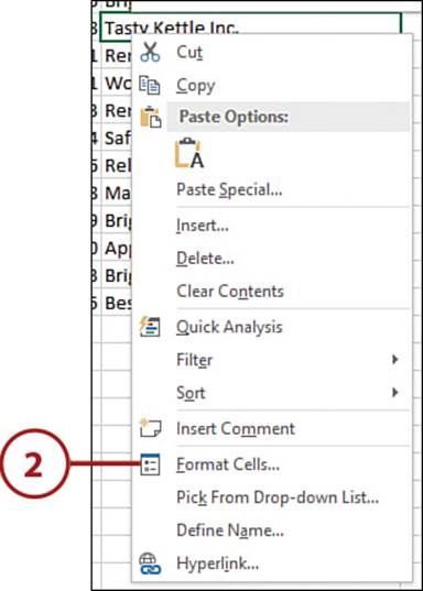
2. Right-click over the selection and select Format Cells.
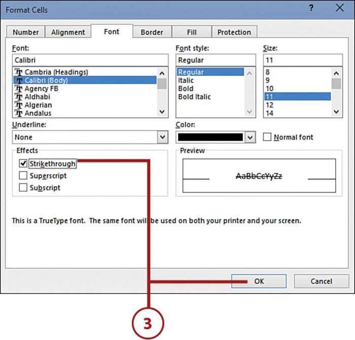
3. Select the desired effect(s) from the Effects group and click OK.
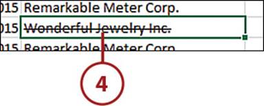
4. The effect will be applied to the selected range.
Change the Font Color
Emphasis can also be added to a range by using color, or you can use color to just make the data look pretty.
1. Select the range for which you want to change the font color.
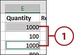
2. On the mini toolbar, open the Font Color drop-down and click on the desired color.
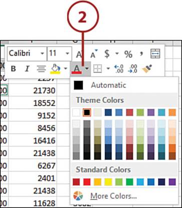
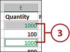
3. The range will update to the selected color.
More Colors
If you don’t see the color you want in the drop-down, click More Colors to open the Color dialog box to access all the colors available. The dialog box will also allow you to enter the RGB and HSL values for colors.
Reapply the Default Color
To quickly return to the default color, usually black, select the Automatic option at the top of the Font Color drop-down.
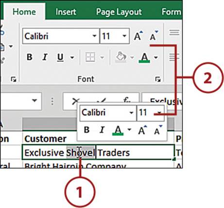
Format a Character or Word in a Cell
You can change the font settings of a single character or word in a cell, not just the entire cell contents.
1. Double-click the cell so that the cursor appears in the cell and you can select the desired character or word.
Select Text in the Formula Bar
You can also select the desired text via the formula bar. Select the cell and then select the character or word in the formula bar.
2. A modified mini toolbar will appear when you are done with the selection and when you right-click over the selected text. You can make selections from this smaller toolbar or make your selections from the options on the Home tab.
Format Quickly with the Format Painter
The Format Painter enables you to quickly copy the formatting of one range to another. Copied formatting includes font, color, and number formatting; it does not include row heights or column widths.
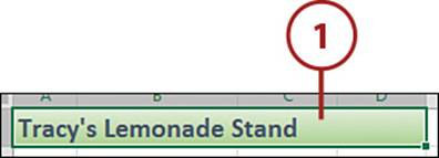
1. Select the range with the formatting to duplicate.
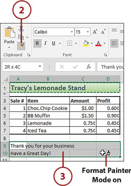
2. Click the Format Painter button. The pointer changes to a paintbrush with a plus sign.
3. Click the cell in the upper-left corner of the destination range if the range is the same size. If the destination range is larger, select the entire range.
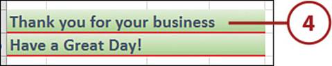
4. The formatting is applied, and the pointer changes back to normal.
Paint Multiple Ranges
By default, the Format Painter is a one-shot tool. To get it to stay on until you are done pasting the formatting everywhere you want to apply it, double-click the Format Painter button. The button will remain on until you press the Esc key or double-click the button to turn it off.
Adjusting the Row Height
If the text is wrapping to the next line in your cell, you might not be able to see all of it. This is especially true if you have merged cells—Excel won’t automatically adjust the row height for merged cells as it will for non-merged cells.
Modify the Row Height by Dragging
You can quickly change the row height by adjusting the line between the row headings.
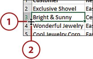
1. Place your pointer on the line below the row heading of the row to resize. For example, if you want to resize row 3, move your pointer onto the line below row 3.
Resize Multiple Rows at a Time
You can resize multiple rows at a time. Select the rows then place the pointer below any row heading in the selection.
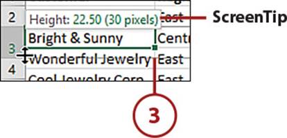
2. When the pointer changes to a two-headed arrow, click and hold down the mouse button.
3. As you drag to resize the row to the desired height, a ScreenTip will appear by the pointer, showing the current height. Let go of the mouse button when you’ve reached the desired height.
Set the Maximum Needed Height
If there are no merged cells in the row to resize, you can use the double-click method to have Excel calculate the required maximum height of the row. When you get the two-headed arrow, double-click and Excel will size the row for you.
Modify the Row Height by Entering a Value
Row heights are based on points. If there are no cells with wrap turned on, then the default row height will be slightly larger than the largest font size in the row. You can change this by entering a specific value.
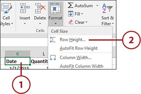
1. Select a cell in the row you want to adjust. Cells in multiple rows can be selected.
2. On the Home tab, select Row Height from the Format drop-down.
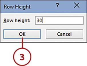
3. Enter the new height and click OK.
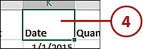
4. The row height will adjust to the new value.
Use Font Size to Automatically Adjust the Row Height
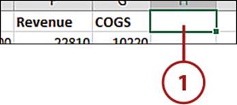
The default row height is based on the largest font size in the row. For example, if cell F2 has a font size of 26, even if there is no other text in the row, the row automatically adjusts to approximately 33 points, providing a little empty space above and below the text. You can take advantage of this to set the height of a row, instead of manually setting the row height. The advantage is that when a user tries autofitting the row height, your setting won’t change.
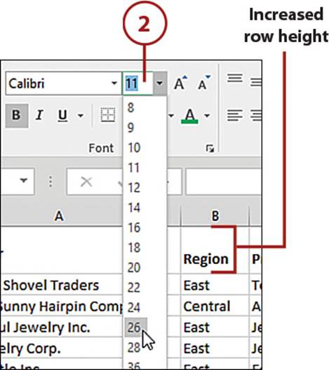
1. Select a blank cell in the row to adjust. You want a cell that won’t ever have text in it, or the text will be that font size.
2. On the Home tab, from the Font Size drop-down, select a new font size.
Height Doesn’t Adjust Completely
If manual height adjustments have been applied to a row, the font size method will not work right away. If that happens, use the double-click method to reset the automatic adjustment functionality for the row.
Adjusting the Column Width
If you can’t see all the data you enter in a cell or the data in a column doesn’t use up very much of the column, you can adjust the column width as needed.
Modify the Column Width by Dragging
You can quickly change the column width by adjusting the line between the column headings.
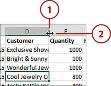
1. Place the pointer on the line to the right of the column heading of the column you want to resize. For example, if you want to resize column D, move your pointer over the line between headings D and E.
Resize Multiple Columns at a Time
You can resize multiple columns at a time. Select the columns and then place the pointer to the right of any column heading in the selection.
2. When the pointer changes to a two-headed arrow, hold down the mouse button.
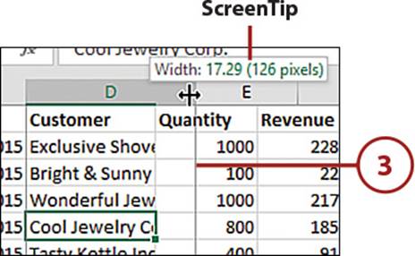
3. As you drag to resize the column to the desired width, a ScreenTip will appear by the pointer, showing the current width. Let go of the mouse button when you’ve reached the desired width.
Set the Maximum Needed Width
If your cells aren’t merged or wrapped, you can use the double-click method to have Excel calculate the required maximum width of the column. When you get the two-headed arrow, double-click and Excel will size the column for you based on the cell with the longest entry.
If you have multiple columns selected, each column will adjust to its own required maximum width.
Modify the Column Width by Entering a Value
You can adjust the column width to a specific value. This value represents the number of characters that can be displayed in a cell formatted with the default font style.
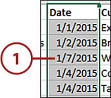
1. Select a cell in the column you want to adjust. Cells in multiple columns can be selected.
2. On the Home tab, in the Format drop-down, select Column Width.
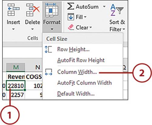
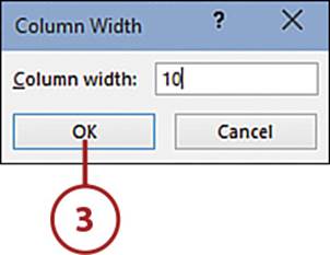
3. Enter the new width and click OK.
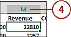
4. The column width will adjust to the new value.
Aligning Text in a Cell
Excel allows you to change the vertical and horizontal alignment of data in a cell. By default, text is left aligned in a cell and numbers are right aligned. Both are bottom aligned.
Change Text Alignment
You can change the horizontal and vertical alignment of text in a cell so that it appears as you need it.
1. Select the range for which you want to change the alignment.
2. On the Home tab, select a vertical and/or horizontal alignment option.
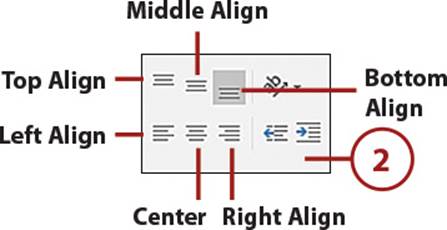
3. The range’s alignment will change to match your selection(s).
Merging Two or More Cells
The process of merging cells takes two or more adjacent cells and combines them to make one cell. For example, if you are designing a form with many data-entry cells and you need space for a large comment area, resizing the column might not be practical because it will also affect the size of the cells above and below it. Instead, select the range you want the comments to be entered in and merge the cells. Any existing text in cells other than the upper-left cell of the selection is deleted as the newly combined cell takes on the identity of this first cell.
It’s Not All Good: Merged Cells Limit Excel
Use caution when merging cells because it can lead to potential issues:
• Users will be unable to sort if there are merged cells within the sort range.
• Users will be unable to cut and paste unless the same cells are merged in the paste location.
• Column and row AutoFit won’t work.
• Lookup-type formulas will return a match only for the first matching row or column.
Merge and Center Data
Excel makes it easy to merge cells and center the data by having a single button that does both these actions right on the Home tab.
1. Select the cells to merge.

2. On the Home tab, select Merge & Center.
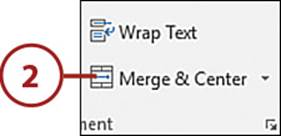
3. The selected cells will merge, and any data in the leftmost cell will be centered.
Merge But Don’t Center
If you want to merge cells but not center the data, open the Merge & Center drop-down and select Merge Cells. The alignment of the leftmost cell in the selection will be applied to the merged cell.
Merge Across Columns
When you select a range that contains both multiple columns and multiple rows, Excel merges the entire range into a single cell. If you want to merge only the columns, creating a separate merged cell in each row, you can use the Merge Across option. This keeps the rows separate but merges the columns.
1. Select the rows and columns you want to merge. You don’t have to select the same number of columns in each row.
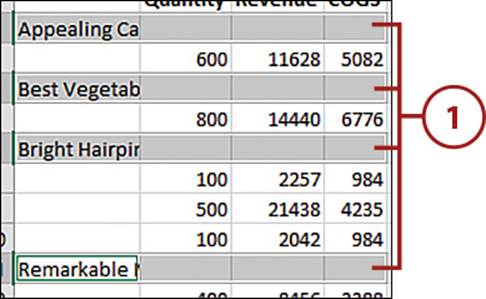
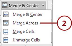
2. On the Home tab, from the Merge & Center drop-down, select Merge Across.
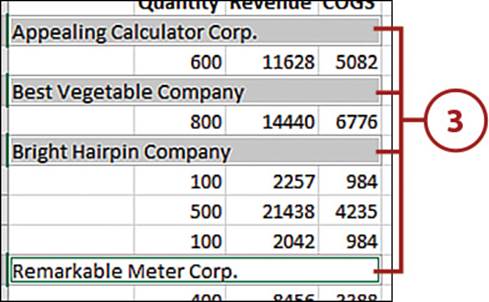
3. The selected columns in each row will be merged together.
Unmerge Cells
Unmerge cells to revert them to their individual state.
1. Select one or more merged cells.
2. On the Home tab, from the Merge & Center drop-down, select Unmerge Cells.

3. The cells will unmerge with any data appearing in the upper-left cell only.
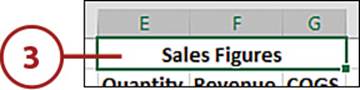
Centering Text Across Multiple Cells
As noted in the earlier section “Merging Two or More Cells,” merging cells can cause problems in Excel, limiting what you can do with a dataset. If you need text to span across several columns, instead of merging the cells, you can center the text across the multiple columns.
Center Text Without Merging
Centering text across a selection gives the illusion of merged cells without the complications.
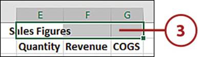
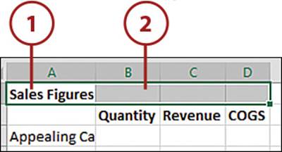
1. Enter your title in the leftmost cell of the dataset.
2. Select the title cell and extend the range to include all cells you want the title centered over.
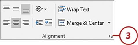
3. From the Home tab, click on the Alignment group’s dialog box launcher.
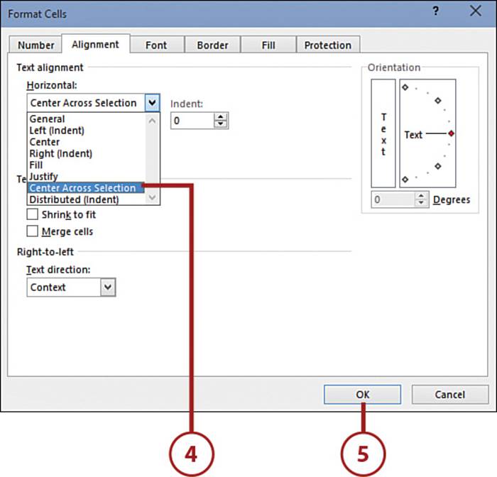
4. From the Horizontal drop-down, select Center Across Selection.
5. Click OK.
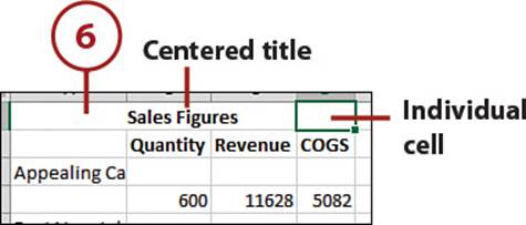
6. The title will be centered above the dataset, but still consists of individual cells.
Wrapping Text in a Cell to the Next Line
When you type a lot of text in a cell, it continues to extend to the right beyond the right border of the cell if there is nothing in the adjacent cell. You can widen the column to fit the text, but sometimes that may be impractical.
Wrap Text in a Cell
Set a cell to wrap text, moving any text that extends past the edge of the column to a new line in the cell.
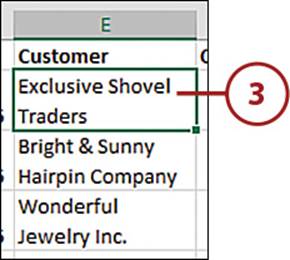
1. Select the range you want to set to wrap.
2. On the Home tab, select Wrap Text.
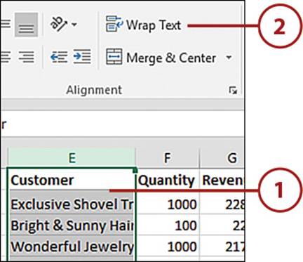
3. The data in the selection will wrap, and the rows will automatically adjust their heights to show the extra lines.
It’s Not All Good: AutoFit Row Height Isn’t Working Right
Normally, when you wrap a cell, the row height automatically adjusts to fit the text. But if you’ve manually adjusted the row height any time before pasting or if you have merged cells, Excel will not autofit the row. If there are merged cells, unmerge them. Then, reset the AutoFit setting by manually forcing an autofit (see the “Adjusting the Row Height” section). The row height will begin to automatically adjust again.
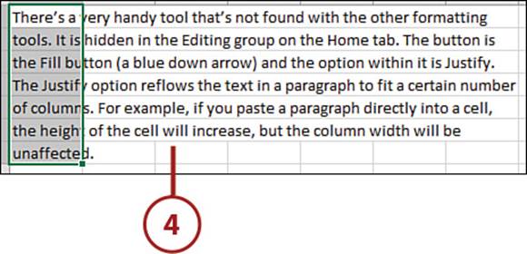
Reflowing Text in a Paragraph
If you paste text into a cell, it may continue to the right, beyond what you can see on your screen. You could manually insert line breaks in the text, or you could flow the text to fit in a selected range.
Fit Text to a Specific Range
You can reflow text so that it uses the specified rows and columns. Unlike wrapped text, this doesn’t affect the row height.
Select a Big Enough Range
Be careful when selecting the range, because if you don’t have enough empty rows available for the text to flow into, Excel will, after warning you, overwrite the rows below the selection.
1. Ensure that the text is contained in a single column of cells. The text can overflow into adjacent columns to the right, but the leftmost column must contain the text and the remaining columns must be blank.
2. Select a range as wide as the finished text should be. Ensure that the upper-left cell of the selection is the first line of text.
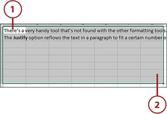
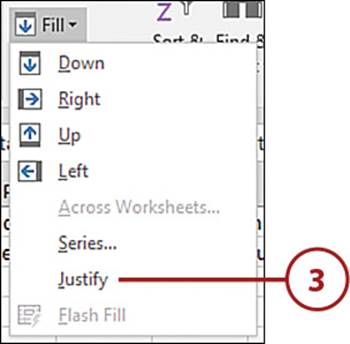
3. On the Home tab, from the Fill drop-down, select Justify.
4. The text reflows so that each line is within the range selected in step 2.
Indenting Cell Contents
By default, text entered in a cell is flush with the left side of the cell, whereas numbers are flush to the right. To move a value away from the edge, you might be tempted to add spaces before or after the value. However, if you change your mind about this formatting at a later time, it can be quite tedious to remove the extraneous spaces.
Indent Data
Use the indent tools instead of spaces to change the indention of data in a cell.
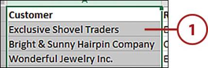
1. Select the range for which you want to change the indent.
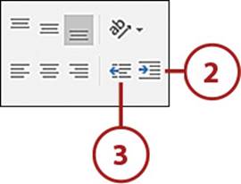
2. Click the Increase Indent button until the data is increased the desired amount.
3. Click the Decrease Indent button to remove an indent.
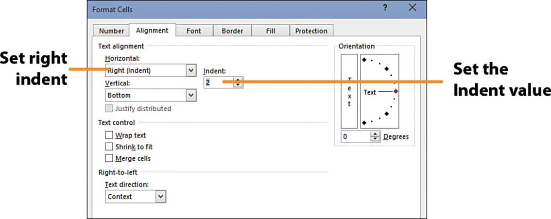
It’s Not All Good: Indenting Right-Aligned Numbers
If you use the indent buttons with a right-aligned number, the number will become left aligned and adjust from the left margin.
To get a right-aligned number to indent from the right side of a cell, go to the Alignment tab of the Format Cells dialog box, set the Horizontal alignment to Right, and then set the Indent value.
Applying Number Formats
The way you see number data in Excel is controlled by the format applied to the cell. For example, you may see the date as August 12, 2015, but what is actually in the cell is 42106. Or you may see 10.5%, but the actual value in the cell is 0.105. This is important because when you’re doing calculations, Excel doesn’t care what you see. It deals only with the actual values.
General is the default format used by all cells on a sheet when you first open a workbook. Decimal places and the negative symbol are shown if needed. Thousand separators are not.
Modify the Number Format
By default, the Number format uses two decimal places but does not use the thousands separator. You can change the number of decimals shown or add a thousands separator, formatting the number as needed.
1. Select the range you want to format.
2. Click Comma Style on the Home tab to add a thousands separator.
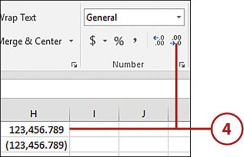
3. Click Increase Decimal to increase the number of decimals shown. You may also have to resize the column to see all the numbers.
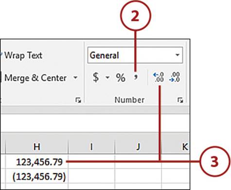
4. Click Decrease Decimal to decrease the number of decimals shown.
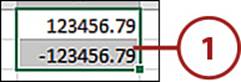
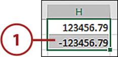
Change the Format of Negative Numbers
Negative numbers can be formatted in a variety of ways: with a leading unary symbol (the dash before a negative number), wrapped in parentheses, or colored red.
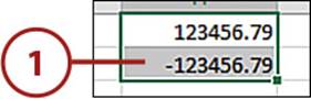
1. Select the range you want to format.
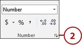
2. From the Home tab, select the Number group’s dialog box launcher.
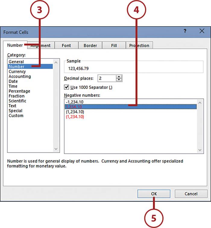
3. On the Number tab, select the Number category.
4. From the Negative Numbers list, select the desired negative number format.
5. Click OK.
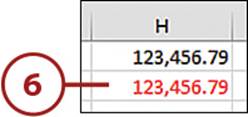
6. Negative numbers will update with the new formatting.
Apply a Currency Symbol
The default currency symbol is based on your Windows settings, but you can use any symbol available.
1. Select the range you want to format.
2. On the Home tab, click Accounting Number Format to apply the symbol shown on the button.
3. To apply a different symbol, open the Accounting Number Format drop-down and choose the desired symbol.
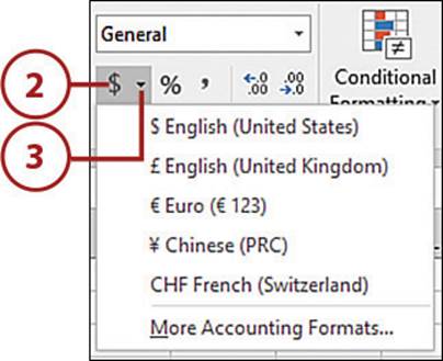
4. The default Accounting number format settings will be applied.
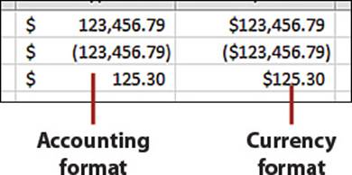
Accounting Format vs. Currency Format
The Accounting and Currency formats are similar in that they both apply a currency symbol, thousands separator, two decimal places, and black negative numbers surrounded by parentheses.
How they differ is in the alignment of the symbol and value. Accounting lines up the currency symbols on the left side of the cell and decimals points to the right side of the cell. Currency places the symbol directly to the left of the value, and the decimal points might not line up.
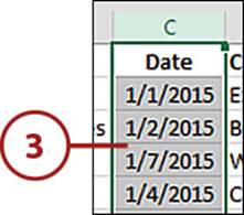
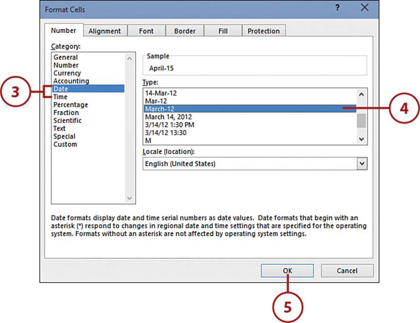
Format Dates and Times
The Number Format drop-down on the Home tab has limited date and time formatting options. More options are available through the Format Cells dialog box, such as showing the date and time together in one cell or showing only the month and year of a date.
1. Select the range you want to format.
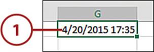
2. On the Home tab, from the Number Format drop-down, select a date or time format. If you don’t see one you like, choose More Number Formats.
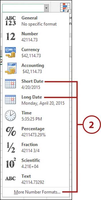
3. Click either the Date or Time category.
4. Scroll through the various types. If you want to see what your data will look like with that format, highlight it and view the sample.
5. Click OK when you’ve found the desired format.
Times in Excel
Excel sees times on a 24-hour clock. That is, if you enter 1:30, Excel assumes you mean 1:30 a.m. But if you enter 13:30, Excel knows you mean 1:30 p.m.
If you need to display times beyond 24 hours, such as if you’re working on a timesheet adding up hours worked, use the time format 37:30:55.
Format as Percentage
When you apply the percentage format, Excel takes the value in the cell, multiplies it by 100, and adds a % symbol at the end. For example, if you have 50 in a cell and apply the percentage format to it, you will see 5000%. If you actually want 50%, you need the decimal value, 0.5, in the cell.
When you use the cell in a calculation, the actual (decimal) value is used. For example, if you have a cell showing 90% and multiply it by 1,000, the result will be (in General format) 900 (0.9*1,000).
Excel Tries to Help
If you include the % symbol when you type the value in the cell, Excel converts the value to its decimal equivalent and then applies the percentage format to the cell.
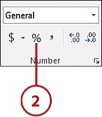
1. Select the range you want to format.
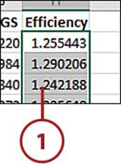
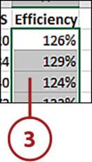
2. On the Home tab, click Percent Style.
3. The values will be multiplied by 100 and a % symbol added.
Format as Text
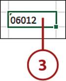
When you type a number with leading zeros into a cell, such as 06012, Excel drops the zero and only 6012 appears in the cell. That’s because real numbers don’t start with zeroes. But there are some cases, such as invoices and ZIP codes, where those leading zeroes are needed. In such cases, you should format the range as text before entering the value.
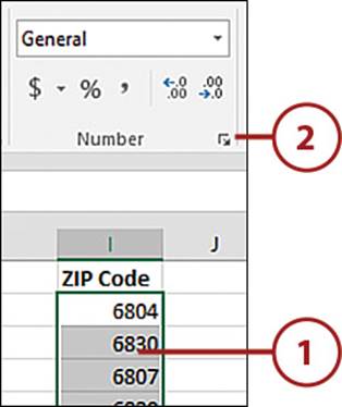
1. Select the range you want to format.
2. On the Home tab, select Text from the Number Format drop-down.
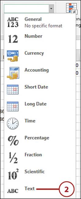
3. Select a cell in the range and type the desired value, such as 06012. The zero won’t get dropped.
Use an Apostrophe Instead
You can also tell Excel you want a number treated as text by typing an apostrophe before the number (for example, ‘06012). One advantage of this method is the cell isn’t converted to the Text format, so if you type a number later on, the number formatting applied to the cell will be retained.
It’s Not All Good: Formatting Existing Values
Excel gets a little strange when it comes to applying the Text format to a cell with numbers in it. If you apply this format to formatted numbers, Excel strips any number formatting from the cell and aligns the number to the left side of the cell. However, you can still use the cells for calculations. The full conversion to “numbers as text” doesn’t happen until you reenter the value in the cell. At this point, you can no longer use the cells for calculations.
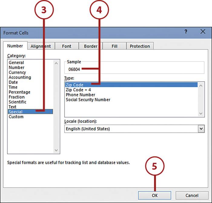
Apply the Special Number Format
The Special category provides formats for numbers that are not actually numbers—ZIP codes, phone numbers, and Social Security numbers. Remember, when you change the formatting of a cell, you change only its appearance. The value in the cell is not affected.
1. Select the range you want to format.
2. From the Home tab, select the Number group’s dialog box launcher.
3. On the Number tab, select the Special category.
4. Select a type. If you want to see what your data will look like with that format, highlight it and view the sample.
5. Click OK when you’ve found the desired format.
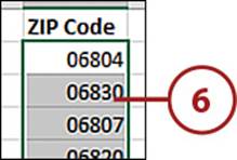
6. The format of your values will update.
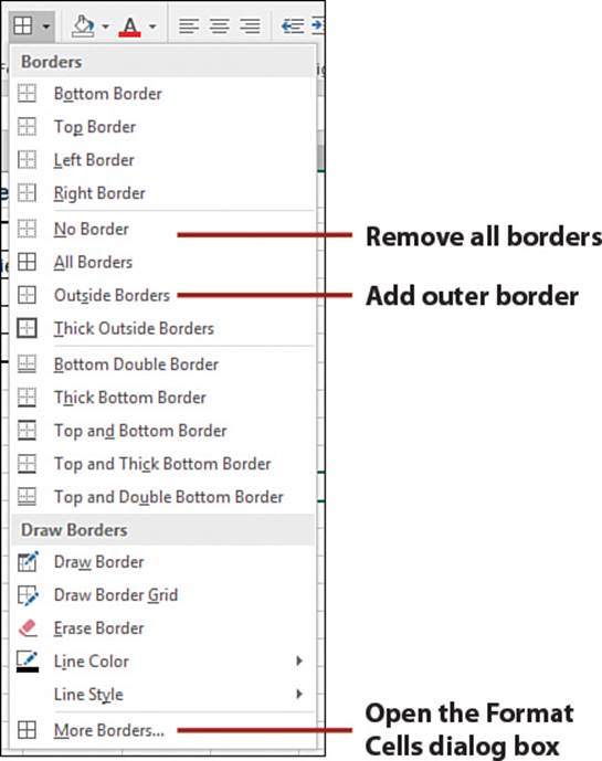
Adding a Border Around a Range
The Borders drop-down on the Home tab includes 13 of the most popular border options. When you’re applying a border, Excel sees the entire selection as one object and applies the border you have chosen to the selection, not the individual cells that make it up. For example, if you select a range consisting of five rows and apply the Bottom Border, the border appears only in the last cell, not at the bottom of each cell in the selection.
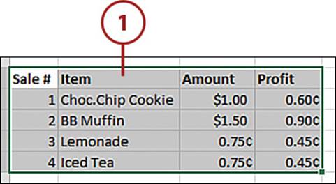
Format a Range with a Thick Outer Border and Thin Inner Lines
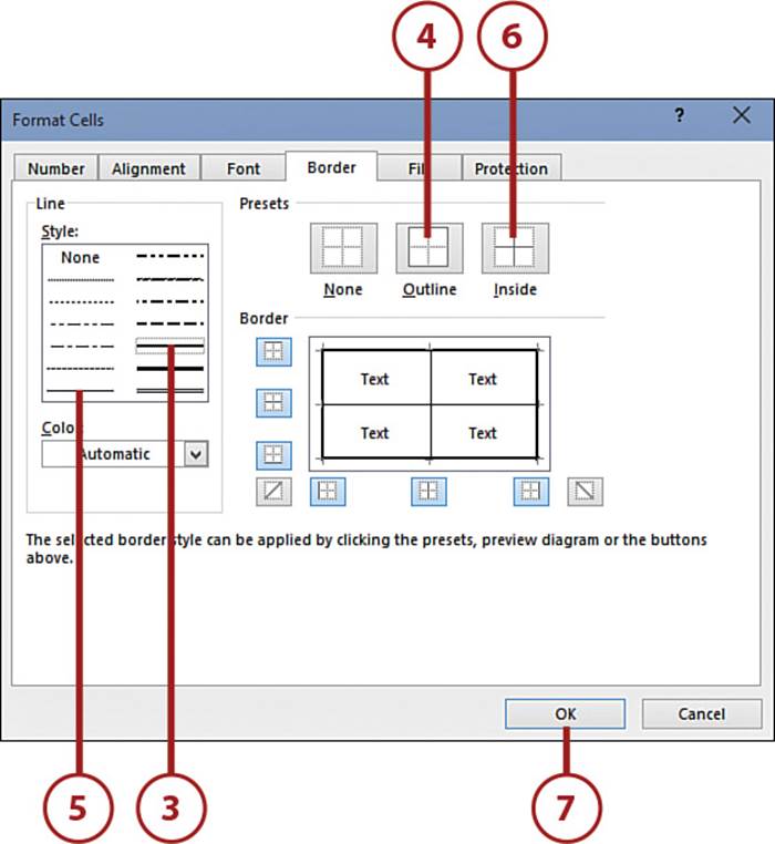
You can apply multiple border formats on top of each other by using the Format Cells dialog box.
1. Select the range to be formatted.
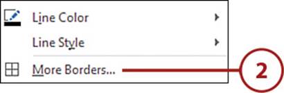
2. Select More Borders from the Borders drop-down.
3. Select a thick border style.
4. Select the Outline preset.
5. Select a thin border style.
6. Select the Inside preset.
7. Click OK.
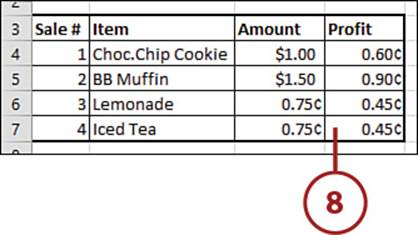
8. The borders will be applied to the selected range.
>>>Go Further: Apply Selective Lines
The Format Cells dialog box allows you to get very specific in the application of borders to a range. You can mix and match the border styles, such as dotted lines and double lines. You can choose where they’re applied within the range, whether it’s the outer border, an inner line, or a diagonal line across the entire range.
Use the sample area of the Format Cells dialog box to build your border design. You can click within the box to add the lines or choose from the buttons surrounding the sample area.
Add a Colored Border
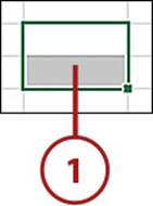
An underline applied to a value underlines only the characters. If you want to cover a larger area—such as the title over a table—apply a bottom border to the cell(s).
1. Select all the cells to which you want to apply the border.

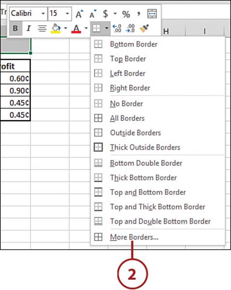
2. Right-click over the selection and select More Borders from the Borders drop-down on the mini toolbar.
3. Select a color from the Color drop-down.
4. Select a thick border style.
5. Click the bottom border button.
6. Click OK.
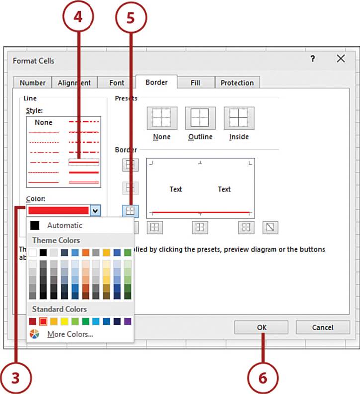
7. The colored border is added to the bottom of the selection.

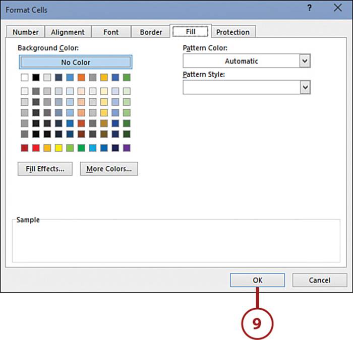
Coloring the Inside of a Cell
Fill color refers to the color applied inside of a cell. You can also apply fill effects, such as patterns, styles, and gradient fills. The pattern color and pattern style work together to fill a cell with a pattern (various dots or lines) in the selected color. This effect is placed on top of the background color.
The Color Palette Has Changed!
You send a workbook to a co-worker and when you get it back, you see a different set of colors in the drop-down. What happened?
In a new, blank workbook, you get the standard color palette. However, Excel allows you to create and share custom color palettes within themes. Themes are good ways to ensure uniformity of color in an organization (see the Chapter 7 section “Using Themes to Ensure Uniformity in Design” for more information).
Apply a Two-Color Gradient to a Cell
A gradient fill is where a color slowly changes from one color to another within a cell. Instead of filling a cell with a single solid color, you can apply a two-color gradient to a range.
1. Select the range you want to format. If you select multiple cells, the gradient will repeat across the range.

2. On the Home tab, select Format Cells from the Format drop-down.
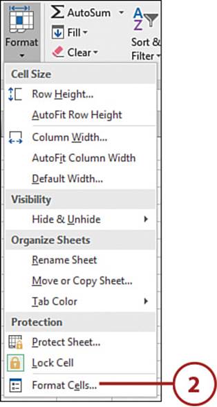
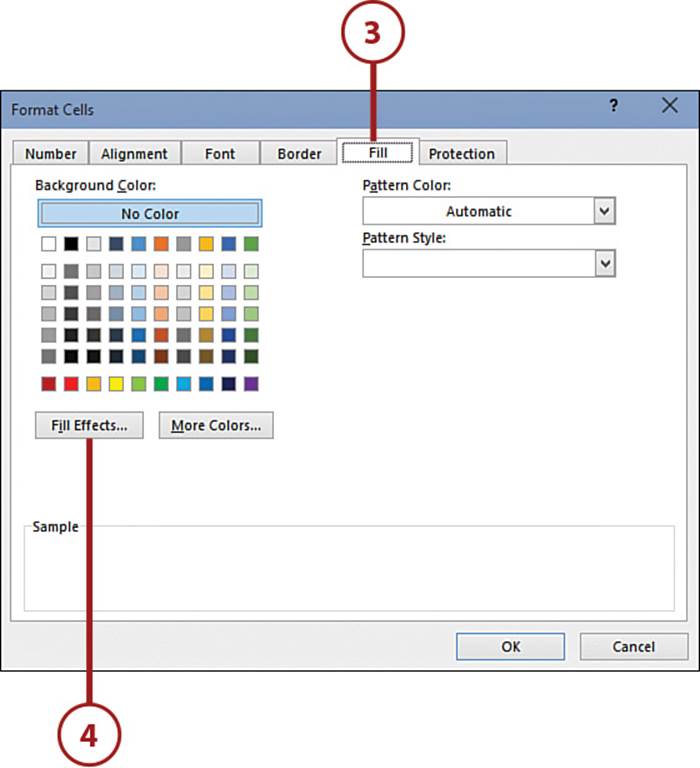
3. Select the Fill tab.
4. Click the Fill Effects button.
5. Select a color from the Color 1 drop-down.
6. Select a different color from the Color 2 drop-down.
7. Select a shading style from the Shading Styles section.
8. Make a selection from the Variants section. The Sample box updates to reflect your selection.
9. Click OK twice.
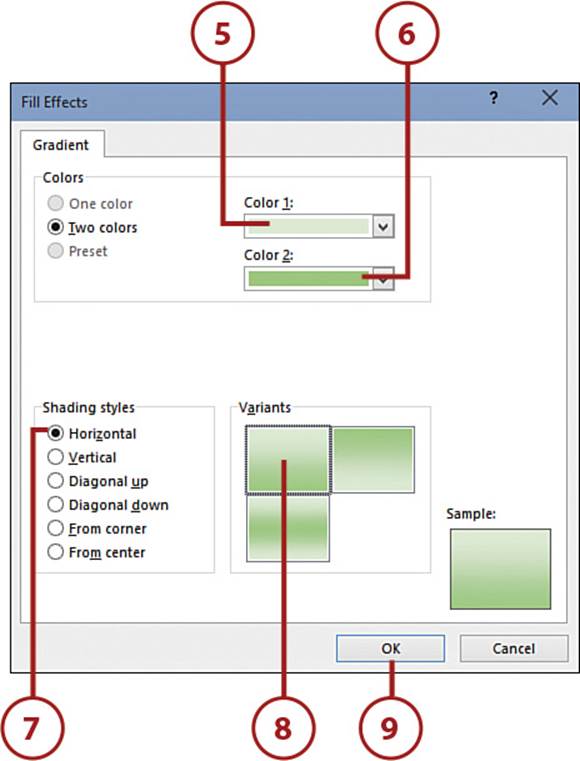
10. The fill effect will be applied to the range.

All materials on the site are licensed Creative Commons Attribution-Sharealike 3.0 Unported CC BY-SA 3.0 & GNU Free Documentation License (GFDL)
If you are the copyright holder of any material contained on our site and intend to remove it, please contact our site administrator for approval.
© 2016-2026 All site design rights belong to S.Y.A.