My Excel 2016 (2016)
8. Using Formulas
Excel is great for simple data entry, but its real strength is its capability to perform calculations. After you design a sheet to perform calculations, you can easily change the data and watch Excel instantly recalculate. This chapter includes the following topics:
→ Entering a formula into a cell
→ Comparing absolute and relative referencing
→ Using array formulas
→ Converting formulas to values
→ Troubleshooting formulas
This chapter not only shows you how to enter a formula, but also teaches you fundamental basics, such as the difference between absolute and relative referencing, which is important when you want to copy a formula to multiple cells, and how to use a name to refer to a cell instead of having to memorize a cell address. You’ll take the formula basics you learn here and apply them later in Chapter 9, “Using Functions,” to really crank up the calculating power of your workbook.
Entering a Formula into a Cell
Typing a formula is similar to entering an equation on a calculator, with one exception. If one of the terms in your formula is already stored in a cell, you can point to that cell instead of typing in the number stored in the cell. The advantage of this is that if that other cell’s value ever changes, your formula automatically updates.
Enter Formula Mode
When the first thing in a cell is an equal sign (=), Excel expects a formula to be entered. If you don’t want to trigger formula mode, type an apostrophe (‘) first.
Calculate a Formula
Use Excel to calculate the tax on items with a 6% tax rate. The item value is already entered in a cell, but you need to type the tax rate into the formula.
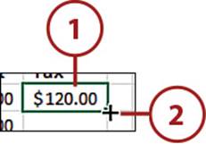
1. Select the cell you want the formula to be in.
2. Type an equal sign (=).
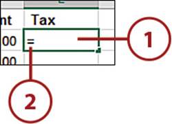
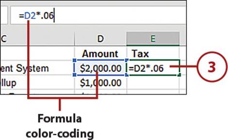
3. Select the cell with the value to include in the formula and then type *.06. The asterisk (*) is the multiplication symbol in Excel. Note that the cell address in the formula and the corresponding highlighted cell have the same color.
Reference Another Sheet
If the range you need to reference is on another sheet in this or another open workbook, simply go to the sheet and select the range. You can continue entering the formula from the other sheet, or return to the original.
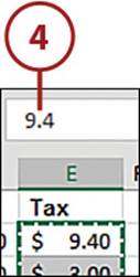
4. Press Enter to complete the formula. Select the cell with the formula to view the formula in the formula bar. It should look like this:
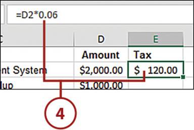
=D2*0.06
>>>Go Further: Order of Operations
Excel evaluates a formula in a particular order if it contains many calculations. Instead of calculating from left to right like a calculator, Excel performs certain types of calculations, such as multiplication, before other calculations, such as addition.
You can override this default order of operations using parentheses. If you don’t, Excel applies the following order of operations:
1. Unary minus (the dash before a negative number)
2. Exponents
3. Multiplication and division, left to right
4. Addition and subtraction, left to right
For example, if you have the formula
=6+3*2
Excel returns 12, because first it does 3*2 and then adds the result (6) to 6. But, if you use parentheses, you can change the order of operations:
=(6+3)*2
This produces 18 because now Excel will do the addition first (6+3) and multiply the result (9) by 2.
View All Formulas on a Sheet
You can toggle between viewing values and formulas on a sheet. To do this, on the Formulas tab, select Show Formulas.

Select All Formulas
If you just want to see what cells have formulas, but don’t need to see the formulas themselves, you can use the Formulas option in the Go to Special dialog box. Press Ctrl+G and click Special to open the dialog box. Select Formulas and click OK, and all formula cells on the sheet will be selected.
Relative Versus Absolute Referencing
When you copy a formula, such as =D2*H1, down a column, the formula automatically changes to =D3*H2, then =D4*H3, and so on. Excel’s capability to change cell D2 to D3 to D4 and so on is called relative referencing. This is Excel’s default behavior when dealing with formulas, but it might not always be what you want to happen.
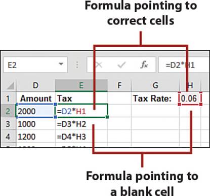
If the cell address must remain static as the formula is copied, you need to use absolute referencing. This is achieved through the strategic placement of dollar signs ($) before the row or column reference.
Lock the Row When Copying a Formula Down
When you copy a formula down a column, the row number increases by one. You can stop this behavior by making the row reference absolute.
1. Select the formula cell.
2. Type a dollar sign ($) to the left of the row number that needs to remain static.
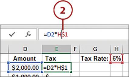
3. Press Enter to calculate the formula.
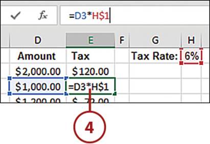
4. Copy the formula down (see “Copy by Dragging the Fill Handle,” later in this chapter). Notice that the row number with the dollar sign does not change.
Lock the Column When Copying a Formula Across
To lock the column when copying a cell across a row, place the $ to the left of the column letter, making the column absolute.
>>>Go Further: Using F4 to Change the Cell Referencing
Instead of typing the $ manually, press the F4 key right after entering the cell address. Each press of the key changes the cell address to another reference variation. For example, if the cell address is A1, the rotation would be A1, $A$1, A$1, $A1, and then back to A1.
If you need to change a reference after you’ve already entered the formula, you can still place the insertion point in the cell address and use the F4 key to toggle through the references.
Copying Formulas
Once you enter a formula, you may want to copy it: across the row, down the column, or to another workbook. You might just have to copy it to a few cells or into thousands of cells. You might want to copy the formula, but not the formatting. There are many combinations of how you might need to copy the formula, and Excel has methods you can use to cover all of them, without retyping the formula.
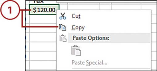
Copy and Paste Formulas
When you copy and paste a formula, not only is the formula pasted, but the formatting of the originating cell is too, unless you choose otherwise. Any relative cell addressing updates accordingly.
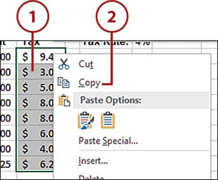
1. Right-click over the cell you want to copy and click Copy.
2. Select the range you want to copy the formula into.
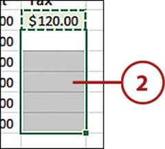
3. Right-click over the selection and click Paste.
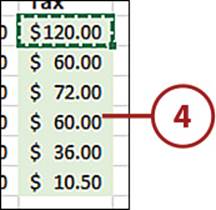
4. The formula and formatting is pasted to the new range.
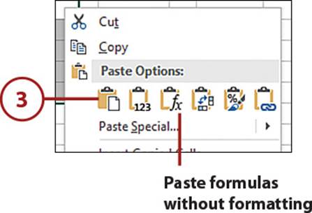
Paste Formulas Without Formatting
If you want to paste the formulas without any of the formatting, use the Formulas option available when you right-click over the selection to paste to. Any relative cell addressing updates accordingly.
Copy by Dragging the Fill Handle
This method is useful if you need to copy your formula across a row or down a column. Any formatting in the originating cell will also be copied.
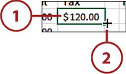
1. Select the cell with the formula.
2. Place your pointer over the fill handle until a black cross appears.
Missing Fill Handle
If you don’t get the fill handle, it’s possible you have the option turned off. Go to File, Options, Advanced and ensure Enable Fill Handle and Cell Drag-and-Drop is selected.
3. Hold the mouse button down as you drag the fill handle. Release the mouse button when you’ve copied the formula to all the desired cells.
Copy Without Formatting
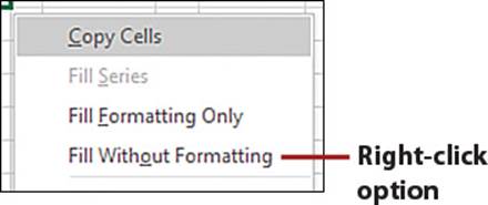
If you hold the right mouse button down as you drag, instead of the left, you can choose Fill Without Formatting, which will copy the formula but not the formatting.
Copy Rapidly Down a Column
If you need to copy a formula into just a few rows, dragging the fill handle is fine. But if you have several hundred rows to update, you could zoom right past the last row. And if you have thousands of rows, using the fill handle can take quite some time.
1. Select the cell with the formula.
2. Place your pointer over the fill handle until a black cross appears.
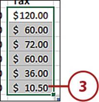
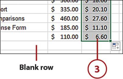
3. Double-click, and the formula will be copied down the sheet until it reaches the end of the dataset (a fully blank row).
It’s Not All Good: Formula Doesn’t Copy All the Way Down
This double-click method relies on having your data set up so that Excel can properly identify it. If Excel can’t figure out the full dataset, then the method won’t work properly.
Excel uses fully blank rows and columns to mark the end of a dataset. You can have a blank cell here and there within the dataset. If you want to test if Excel will properly identify the dataset, select a cell within it and press Ctrl+A. If you see any blank columns or rows interfering with the desired selection, add some temporary text and then try the selection again.
Copy Between Workbooks Without Creating a Link
Sometimes when you copy a formula from one workbook to another, a link to the source workbook is created in the target workbook. This is most common when the formula includes names or links to other sheets. You’ll have to do things a little differently if you don’t want that link.
1. Select the cell with the formula.
2. Highlight the formula in the formula bar. This places Excel in Edit mode, so be careful not to make unwanted changes.
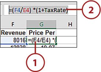
Resize the Formula Bar
If you can’t see the entire formula, click the down arrow at the right end of the formula bar. This will make the formula bar taller. Click the arrow again to shrink the bar back to normal.
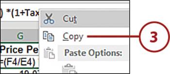
3. Right-click over the formula bar selection and click Copy. Press Esc on the keyboard to exit Edit mode.
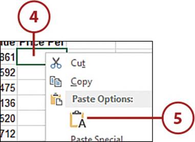
4. Select the cell in the target workbook where you want to paste the formula.
5. Right-click over the cell and click Paste.
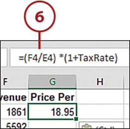
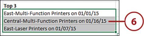
6. The formula will paste exactly as you copied it. When you copy a formula in this way, it’s like copying text, so Excel does not update any relative cell addresses or link to the original file.
Converting Formulas to Values
Formulas take up a lot of memory, and the recalculation time can make working in a large workbook a hassle. At times, you need a formula only temporarily; you just want to calculate the value once and won’t ever need to calculate it again. You could manually type the value over the formula cell, but if the result is a long number, or if you have a lot of calculation cells, this isn’t convenient.
Paste as Values
Use paste options to get rid of formulas, but retain values and formatting.
1. Select the range of formulas.
2. Right-click over the selection and click Copy.
3. With the range still selected, right-click over it and select Values.
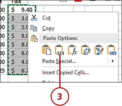
4. The formulas will be replaced with the calculated values.
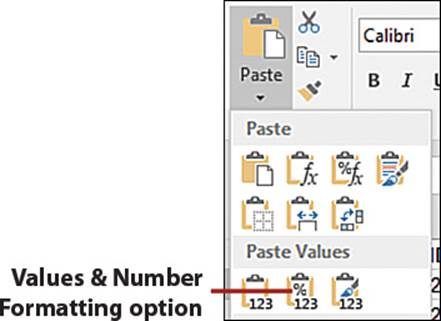
Keep Numeric Formatting
If you want to keep the numeric format, use the Values & Number Formatting option available in the Paste drop-down on the Home tab.
Select and Drag
This method is quite a bit faster than the previous.
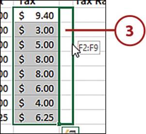
1. Select the range of formulas.
2. Place your pointer on the edge of the dark border around the range so that it turns into a four-headed arrow.

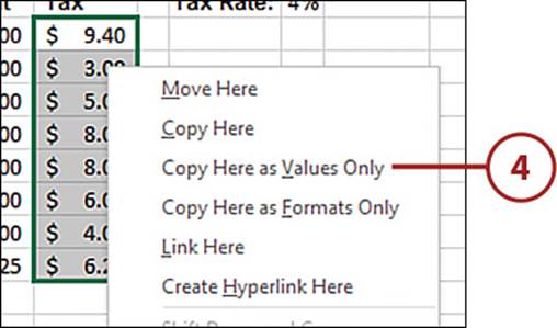
3. Hold the right mouse button down and drag the range to the next column and then back to the original column. Release the right mouse button and a special right-click menu will appear.
Location Matters
Be very careful that you place the range exactly where it was originally. Excel allows you to use this method to place the range in a new location.
4. Select Copy Here as Values Only.
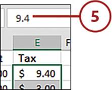
5. The formulas will be replaced with the calculated values.
Using Names to Simplify References
It can be difficult to remember what cell you have a specific entry in when you’re writing a formula. And if the cell you need to reference is on another sheet, you have to be very careful writing out the reference properly, or you must use the mouse to go to the sheet and select the cell.
Instead of remembering a cell address, use a name, such as TaxRate, in your formula. After a name is applied to a range, any references to the range can be done by using the name instead of the address.
Create a Named Cell
Quickly create a name to make it easier to reference a range.
1. Select the range you want to apply the name to.
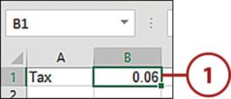
2. In the Name Box, type in the name. It cannot contain spaces.
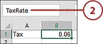
3. Press Enter for Excel to accept the name. Whenever you select the range, you will see the name instead of a cell address in the Name Box.
>>>Go Further: Rules for Creating Names
You only need to remember a few limitations when creating a name:
• The name must be one word. You can use an underscore (_), backslash (\), or period (.) as a spacer.
• The name cannot be a word that might also be a cell address. This was a real problem when people converted workbooks from legacy Excel to Excel 2007 or newer because some names, such as TAX2009, weren’t cell addresses before. Now in Excel 2007 and newer versions, such names cause problems when you open a legacy workbook. So name carefully!
• The name cannot include any disallowed characters, such as a question mark (?), exclamation mark (!), or hyphen (-). The only valid special characters are the underscore (_), backslash (\), and period (.).
• Names are not case sensitive. Excel will see “sales” and “Sales” as the same name.
• You should not use any of the reserved words in Excel, even though Excel will let you. These words are Print_Area, Print_Titles, Criteria, Database, and Extract.
Use a Name in a Formula
Once you create a name, you’ll want to use it in new or existing formulas.
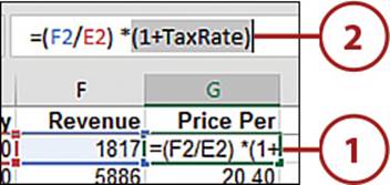
1. Select the cell with the formula.
2. In the formula bar, highlight the cell address you want to replace.
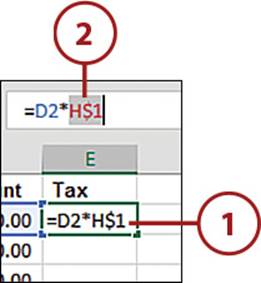
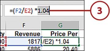
3. Type the name and press Enter to update the formula.
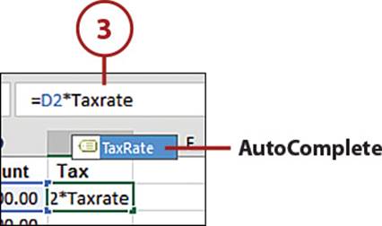
AutoComplete Box
As you type the name, an AutoComplete Box appears. When you see the name, you can select it either with the mouse or by highlighting it and pressing Tab.
>>>Go Further: Global Versus Local Names
Names can be global, which means they are available anywhere in the workbook. Names can also be local, which means they are available only on a specific sheet. With local names, you can have multiple references in the workbook with the same name, but they will only work on the sheet they’re scoped to. Global names must be unique to the workbook. If you don’t specify a sheet when creating a name, the name will be global.
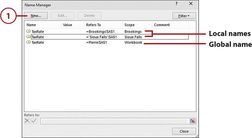
The Name Manager dialog box (click Name Manager on the Formulas tab), lists all the names in a workbook, even a name that has been assigned to both the global and local levels. The Scope column lists the scope of the name, whether it is the workbook or a specific sheet such as Brookings.
If you have a name that is scoped both globally and locally, Excel will automatically reference the global name, unless you are referencing the local name on the sheet on which it resides. In that case, Excel will let you choose which scope you want to reference.
You can create a local name from the Name Manager.
1. Click New.
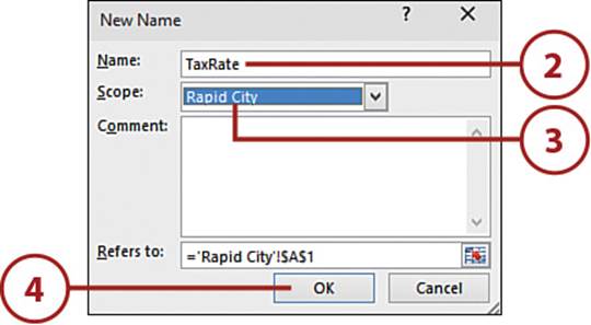
2. Enter the name.
3. Select the sheet to which it should be scoped.
4. Click OK.
Inserting Formulas into Tables
Names are automatically created when you define a table. A name, or a specifier, for each column and the entire table is created. Just like you can use names to simplify references in your standard formulas, you can use specifiers to simplify references to the data in your table formulas.
Define a Table
See the “Define a Table” section in Chapter 4, “Getting Data onto a Sheet,” for information on defining a table.
Write a Formula in a Table
Excel uses the column specifier instead of the cell address when you reference table cells in your formulas.
1. If you don’t already have a column ready for the formula, add one by typing a header in a new column adjacent to the table. Excel will automatically extend the table to include the new column.
2. Select the first data cell in the column.
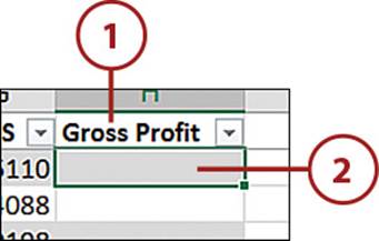
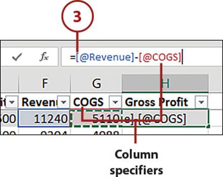
3. Type an equal sign (=) and then select the first cell in the formula. You will notice that column specifiers are used in the formula instead of cell addresses. Enter the rest of the formula.
When You See a Cell Address
If you select a cell in a different row than that of the formula cell, you will see a cell address. Excel expects formulas in a table to reference the same row or an entire column or table.
4. Press Enter, and Excel copies the formula down the column of the table. Notice the formula is the same in every cell.
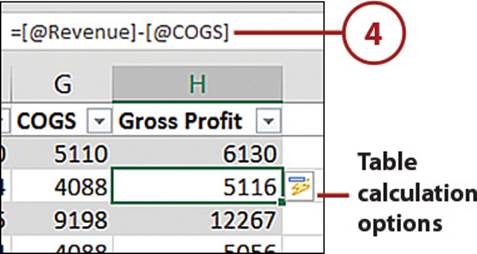
Table Calculation Options
After you enter the formula, a lightning bolt drop-down appears by the cell. If you don’t want the formula copied down the column, select Undo Calculated Column or Stop Automatically Creating Calculated Columns.
If you stop the process, you will have to turn the option back on under the AutoCorrect options. To do this, go to the File tab, select Options, Proofing, AutoCorrect Options, and on the AutoFormat As You Type tab, select Fill Formulas in Tables to Create Calculated Columns.
Write Table Formulas Outside the Table
Writing formulas with specifiers is very handy, and the ability isn’t limited to formulas within tables.
1. Select a cell outside the table where you want to place the formula. The cell should not be adjacent to the table; otherwise, Excel will make it part of the table.
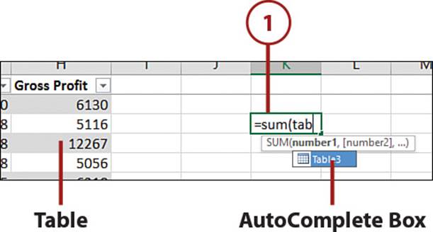
2. Begin entering the formula. When you get to the point where you want to refer to a table component, type the name of the table. You can type the entire name or press Tab when you see it highlighted in the AutoComplete Box.
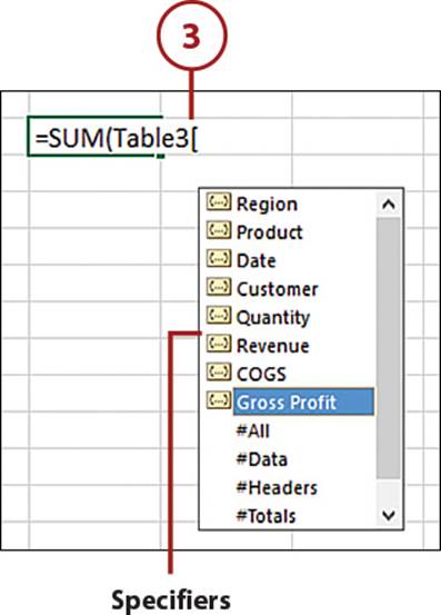
3. Type a left square bracket. A list of specifiers, including the column headers, will appear. Highlight the desired specifier, or type it in, and press Tab.
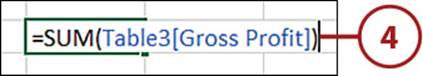
4. Type the closing bracket, finish entering the formula, and press Enter. The formula will calculate.
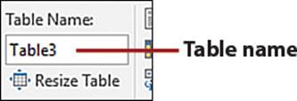
Find the Table Name
Select a cell in the table and click the Table Tools, Design tab. The table name appears in the Table Name field. Use this name in formulas to reference the entire table.
>>>Go Further: More Rules and Specifiers
Besides starting the table reference with the table name and enclosing specifiers in square brackets (TableName[Specifier]), you have a few more rules to keep in mind:
• If you’re using multiple specifiers, each specifier must be surrounded by square brackets and separated by commas. The entire group of specifiers used must be surrounded by square brackets, like this:
TableName[[Specifier1],[Specifier2]]
• To create an absolute reference to a column, refer to the specifier twice, separated by a colon and surrounded by square brackets, like this:
TableName[[Specifier1]:[Specifier1]]
• If no specifiers are used, the table name refers to the data rows in the table. This does not include the headers or total rows.
In addition to the table and column specifiers, Excel provides five more to make it easier to narrow down a particular part of a Table:
• #All—Returns all the contents of the Table or specified column.
• #Data—Returns the data cells of the Table or specified column.
• #Headers—Returns all the column headers or that of a specified column.
• #Totals—Returns the Total Rows or the total of a specified column. If the Total Row option is not on for the table, a #REF error is returned.
• @ – This Row—Returns the current row in which the formula is being typed.
You can combine these specifiers with the column specifiers. For example, to return the total of a column, if Total Rows is on, you could do this:
=TableName[[#Totals][Column Specifier]]
Using Array Formulas
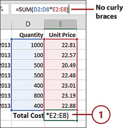
An array holds multiple values individually in a single cell. An array formula allows you to do calculations with those individual values.
You can tell if a formula is an array formula because it’s surrounded by curly braces ({}). These braces are not typed in. They appear after you press Ctrl+Shift+Enter (CSE). If you edit the formula, the braces will go away and you’ll have to press the CSE combination to get them to come back, or press Esc to exit the cell and undo any changes.
Enter an Array Formula
1. If you’re typing the formula, select a cell and enter the formula. Do not press Enter or Tab. Do not type the curly braces ({}).
Or
2. If you’ve copied the formula from another source, double-click the cell so the insertion point is in the cell and then paste the formula. Do not press Enter or Tab. Also, make sure you didn’t include the curly braces ({}) when you copied the formula.
3. Press Ctrl+Shift+Enter (CSE). Excel will place the curly braces around the entire formula and calculate it. Any time you edit the formula, remember to press the CSE combination instead of Enter or Tab when you are done.

Multicell Array Formulas
If you need to return multiple values from the array formula, select the range the formula needs to be in before entering the formula. Once you press the CSE combination, the formula will be copied into the entire range. In some ways, the range will be treated like a single cell. A change in the formula in one cell will affect all the other cells in the range. You won’t be able to insert rows or columns within the range, nor will you be able to move just a part of it.
Delete a Multicell Array Formula
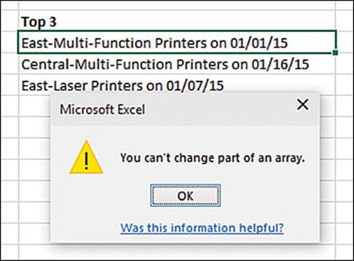
A normal array formula can be cleared like any other formula, but you cannot delete just one cell of a multicell array formula. The message “You can’t change part of an array” will appear if you try to delete just a portion of the range containing the formula. The entire range containing the array formula must be selected before you can delete it.
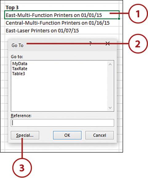
1. Select a cell in the multicell array range.
2. Press Ctrl+G to bring up the Go To dialog box.
3. Click the Special button.
4. Select Current Array.
5. Click OK.
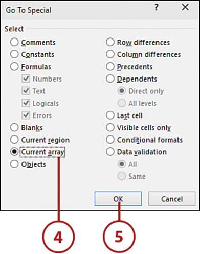
6. The entire array formula range is selected. Press Delete to delete it.
Resize a Multicell Array
If you need to resize a multicell array, you have to delete its entire range, select the new range, and re-enter the formula. You can extend the formula to more cells, but the new cells won’t be part of the original range. If you make a change to the formula in the original range, the change won’t extend to the new cells.
Working with Links
A link is created when a formula in a cell references a range in another workbook or when a chart is copied between workbooks. A link can sometimes be created when you copy a formula from one workbook to another. The workbook that receives information from other sources is the one that is considered linked and will generate prompts to update the data when it is opened.
Invisible Links
If the link is in a formula in a name, instead of a formula in a cell, Excel will not prompt to update the link. The Edit Links option will not be available, either. However, if that name is then used in a cell formula, the prompt and Edit Links option will become available.
Control the Prompt
You can control whether the prompt appears and whether the link is updated when the workbook is opened.
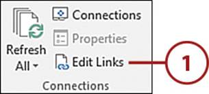
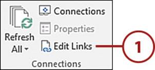
1. On the Data tab, select Edit Links.
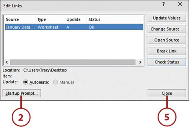
2. Select Startup Prompt.
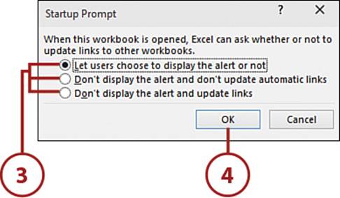
3. Select the desired option.
4. Click OK.
5. Click Close.
Refresh Data
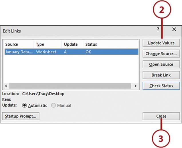
If you didn’t update the link when the workbook first opened but now want to, or you need to force a refresh, you can choose to update the values.
1. On the Data tab, select Edit Links.

2. Click Update Values.
3. Click Close.
Recalculate a Single Cell
To update a single cell, force it to recalculate by double-clicking the cell and then pressing Enter or Tab.
Change the Source Workbook
You don’t have to recreate your linked formulas if the referenced cells are in another workbook. As long as location of the cell is the same, you can just point Excel to the new file.
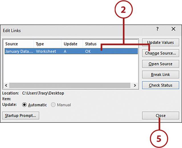
1. On the Data tab, select Edit Links.
2. Highlight the source you want to change and select Change Source.
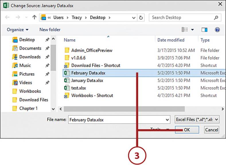
3. Select another workbook and click OK.
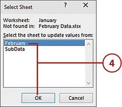
4. If a source sheet isn’t found, Excel will give you the chance to select a new one. Select it and click OK.
5. Click Close.
Break the Link
You can break the formula links, replacing the formulas with the calculated values.
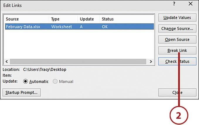
1. On the Data tab, select Edit Links.

2. Select Break Link.
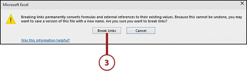
3. Excel warns you that the formulas will be lost and that this action cannot be undone. Click Break Links to continue.
4. Any cell formulas with links to external workbooks will be replaced with just the values. This will not affect named ranges with formulas.
Keep the Formulas
If you want to break the link to the source workbook but keep the formulas intact, you can point the links to the linked workbook itself. Use the Change Source option and select the active workbook. Keep in mind that the active workbook must contain any sheets and named ranges that the source had, else, the action will generate errors.
Troubleshooting Formulas
It can be frustrating to enter a formula and have it return either an incorrect value or an error. An important part of solving the problem is to understand what the error is trying to tell you. After you have an idea of the problem you’re looking for, you can use several tools to look deeper into the error.
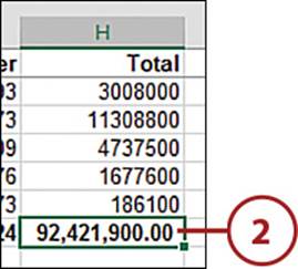
Fix ###### in a Cell
This isn’t usually an error but a matter of the column being too narrow.
1. If your formula isn’t dealing with dates, increase the column width by placing your pointer between column headings and clicking and dragging the column wider.
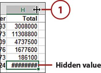
2. When the column is wide enough, the data will be displayed.
Understand a Formula Error
Excel returns different errors depending on what’s causing the issue.
Function Errors
If your formula contains a function, look up the function in the Help to get specific details on what the error means.
1. Select the cell with the error.
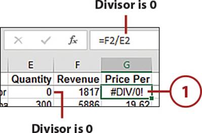
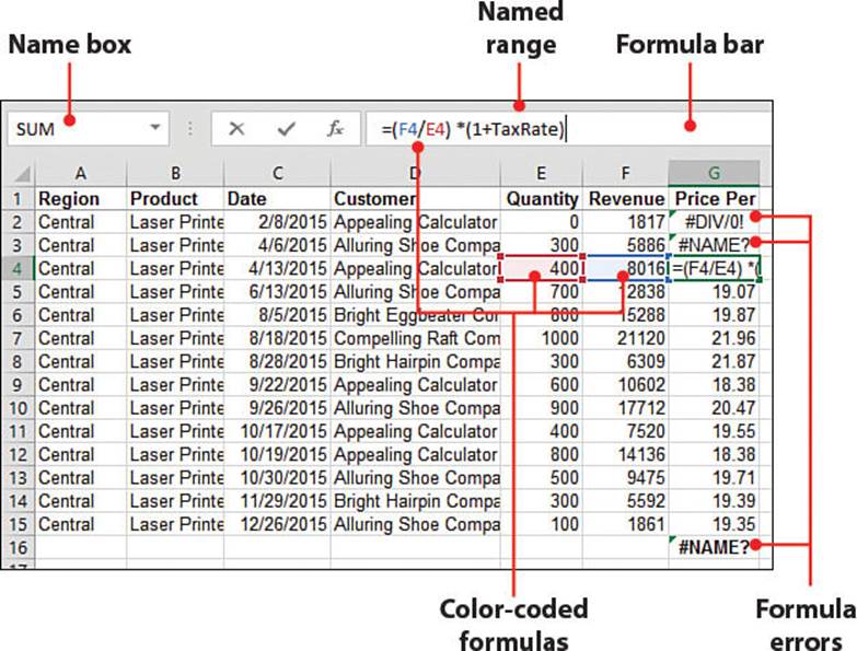
2. If the error is #DIV/0!, a value in the cell is being divided by a 0. If the divisor is a cell, look at that cell and check that it is correct and not zero or blank.
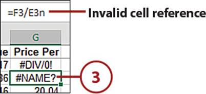
3. If the error is #NAME?, Excel is unable to resolve a reference in the formula (for example, a mistyped name or nonexistent cell address).
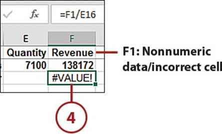
4. If the error is #VALUE!, the formula is trying to do math with nonnumeric data.
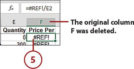
5. If the error is #REF!, a cell reference isn’t valid. The cell has likely has been deleted. There’s no direct way to trace back to the original reference.
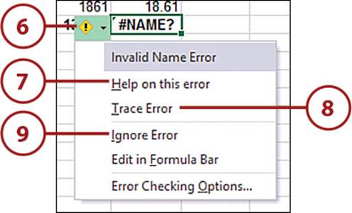
6. If you’re unable to see the issue from looking at the formula, click the exclamation icon next to the formula.
7. Select Help on This Error to open the Excel Help dialog box for more information on the error.
8. Select Trace Error to have Excel highlight the cells used in the formula. See the “Trace Precedents and Dependents” section for more information on using this tool.
Show Calculation Steps Instead of Trace Error
Select Show Calculation Steps to open the Evaluate Formula dialog box. See the “Use the Evaluate Formula Dialog Box” section for information on using this dialog box.
9. Select Ignore Error to hide the error icon. It will reappear if the formula is edited.
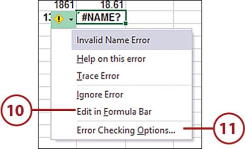
10. Select Edit in Formula Bar, and the insertion point will be placed in the formula bar, highlighting any cells in the formula that are on the active sheet.
11. Select Error Checking Options to open the Options dialog box to the Formulas section, where you can modify how Excel interacts with you when it comes to errors.
Missing Error Icon
If the error icon is not appearing by cells with errors, it’s possible that error checking in Excel has been turned off. To check, and turn it back on, go to File, Options, Formulas and select Enable Background Error Checking. If the option is checked, it’s possible that all errors have been ignored. In that case, click the Reset Ignored Errors button.
Use Trace Precedents and Dependents
Use Trace Precedents to locate cells used by the selected formula. Use Trace Dependents to find out if the selected cell is used in a formula in another cell. When you click one of the trace buttons, arrows appear, linking the cell to other cells.
1. Select the cell you want to trace.
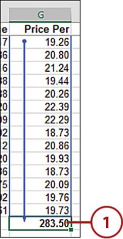
2. To see what cells the selected formula references, click Trace Precedents on the Formulas tab.
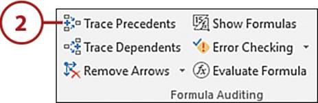
3. Arrows will appear, pointing from the cells used in the formula to the formula cell.
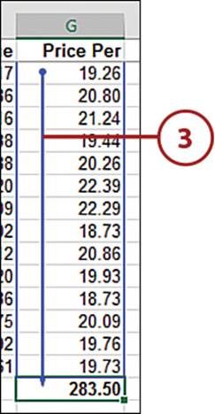
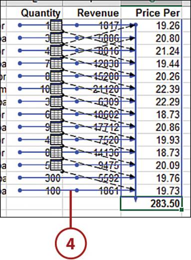
4. Click the button again to see if there are precedents to these cells.
5. To see what formulas the selected cell is used in, click Trace Dependents on the Formulas tab. Arrows appear, pointing from the selected cell to the formulas using it.
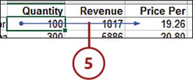
6. Click the button again to see if there are dependents to these cells.
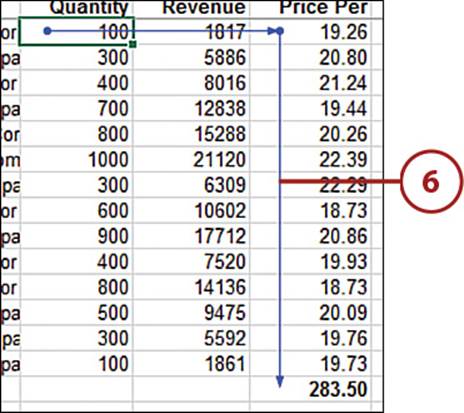
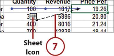
7. If one of the arrows has a dashed line with a sheet icon, the referenced cell is on another sheet. Double-click the dashed line to follow the trace.
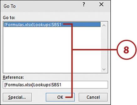
8. Select a reference to inspect and then click OK. Excel will activate the sheet the reference is on and select the cell.
Clear Arrows
To clear all the arrows, select Remove Arrows. To remove precedent arrows, click the Remove Arrows drop-down and select Remove Precedent Arrows. To remove dependent arrows, select Remove Dependent Arrows.
Track Formulas on Other Sheets with Watch Window
The Watch Window allows you to watch a cell update as you make changes to other cells that will affect it.
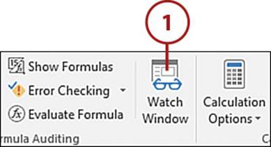
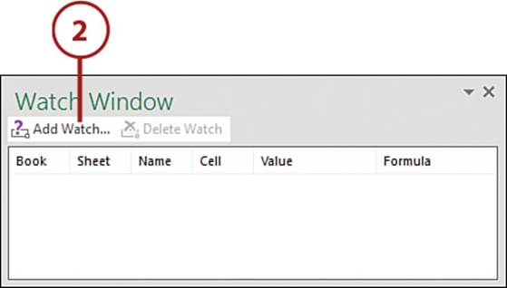
1. On the Formulas tab, click Watch Window.
2. Click Add Watch.
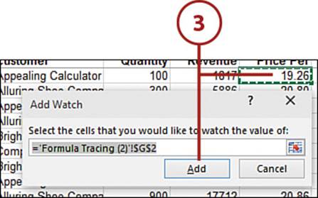
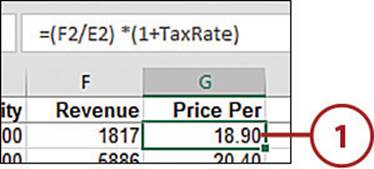
3. Select the cell you want to watch update and click Add.
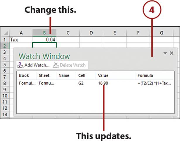
4. Leave the Watch Window open (you can drag it out of the way) and make changes to cells that will affect the watched cells. The Watch Window will update as Excel recalculates.
Use the Evaluate Formula Dialog Box
Use Evaluate Formula to watch how Excel calculates each part of a formula.
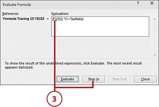
1. Select the formula cell.
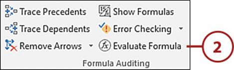
2. On the Formulas tab, select Evaluate Formula.
3. Click Step in to have the underlined portion evaluated.
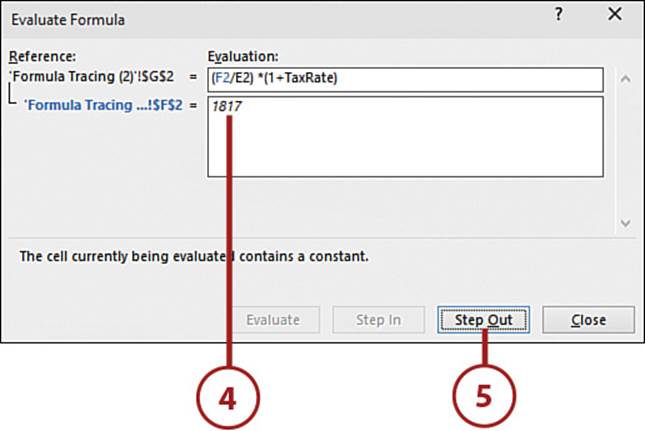
4. The value appears in the second window.
5. Click Step Out.
6. The calculated value replaces its reference.
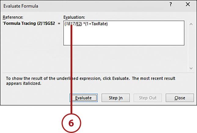
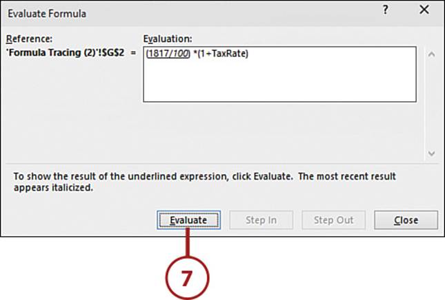
7. You can continue to step in and out, or jump ahead by clicking Evaluate to calculate the underlined portion.
8. If there are additional portions to calculate, repeat the previous steps until the entire formula is evaluated.
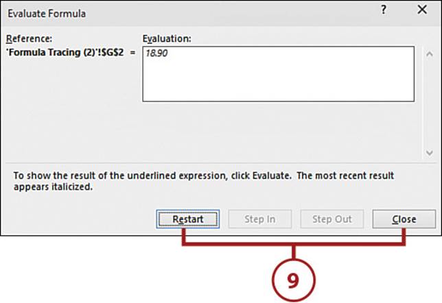
9. Click Restart to go through the steps again, or click Close to return to Excel.
Evaluate with F9
Use F9 to instantly evaluate the highlighted portion of a formula.
1. Select the formula cell.
2. In the formula bar, highlight the part you want to evaluate, including any relevant parentheses. Excel will be in Edit mode.
3. Press F9. The highlighted portion will calculate.
4. To exit Edit mode, press Esc. If you don’t, Excel replaces your formula with the value you just evaluated to.
Adjusting Calculation Settings
By default, Excel recalculates whenever you open or save a workbook, or make a change to a cell used in a formula. At times, this isn’t convenient—such as when you’re working with a very large workbook with a long recalculation time. In times like this, you will want to control when calculations occur. The setting is saved with each workbook.
Set Calculations to Manual
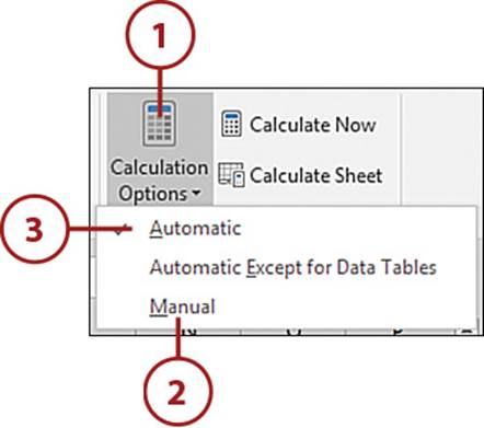
When you set calculations to manual, formulas will only calculate when you first insert them or edit them.
1. On the Formulas tab, click the Calculation Options drop-down.
2. Select Manual.
3. To turn calculations back to automatic, return to the drop-down and select Automatic.
All materials on the site are licensed Creative Commons Attribution-Sharealike 3.0 Unported CC BY-SA 3.0 & GNU Free Documentation License (GFDL)
If you are the copyright holder of any material contained on our site and intend to remove it, please contact our site administrator for approval.
© 2016-2026 All site design rights belong to S.Y.A.