My Excel 2016 (2016)
9. Using Functions
This chapter shows you how to look up functions available in Excel and reviews some functions helpful for everyday use. Goal Seek is also introduced. Other tasks in this chapter include the following:
→ Using the Function Arguments dialog box
→ Using multiple criteria to look up values
→ Calculating the number of workdays between two dates
→ Creating formulas using multiple functions
→ Troubleshooting formulas
A function is like a shortcut for using a long or complex formula. If you’ve ever summed cells using
=A1+A2+A3+A4+A5
you could have instead used the SUM function, like this:
=SUM(A1:A5).
Understanding Functions
Excel offers more than 400 functions. These include logical functions, lookup functions, statistical functions, financial functions, and more.
More Functions
Only a handful of Excel’s functions are reviewed here. For a more in-depth review of functions and possible scenarios you’d use them in, see Excel 2016 In Depth, by Bill Jelen (ISBN 978-0-7897-5584-1).
Look Up Functions
You can always search Excel’s Help to find a function, but you may get more than just the function information you’re looking for. Instead, narrow down the results by using tools provided to specifically search for functions.
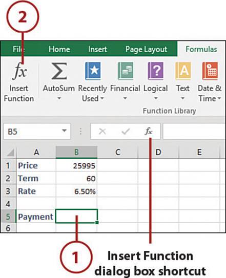
1. Select the cell in which you want the function to appear.
2. On the Formulas tab, select Insert Function.
The Other fx Button
To the left of the formula bar is the symbol fx. This symbol is actually a button that opens the Insert Function dialog box.
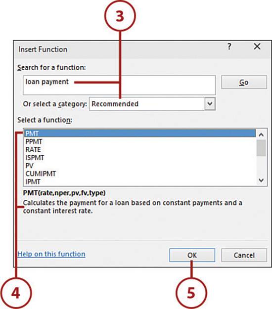
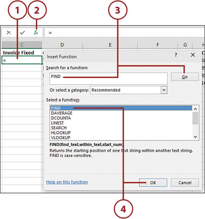
3. Enter a search term in the Search for a Function field or select a category from the drop-down.
4. Select a function from the list box and review the description.
5. Click OK.
6. The function will appear in the active cell, and the Function Arguments dialog box will appear to help you fill in the rest of the arguments.
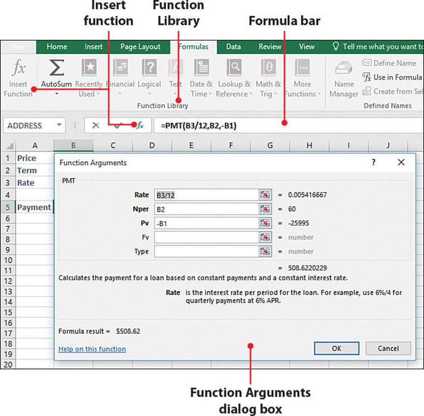
Use the Function Arguments Dialog Box
The Function Arguments dialog box assists in entering the arguments for a selected function. A field exists for each argument. If the function has a variable number of arguments, like the SUM function, a new field will be automatically added when needed.
1. Select the cell that will hold the formula.
2. Click the Insert Function (fx) button by the formula bar.
3. If you know the name of the function, such as FIND, type it in. If not, refer to the section “Look Up Functions.” Select Go.
4. Select the desired function from the list and click OK.
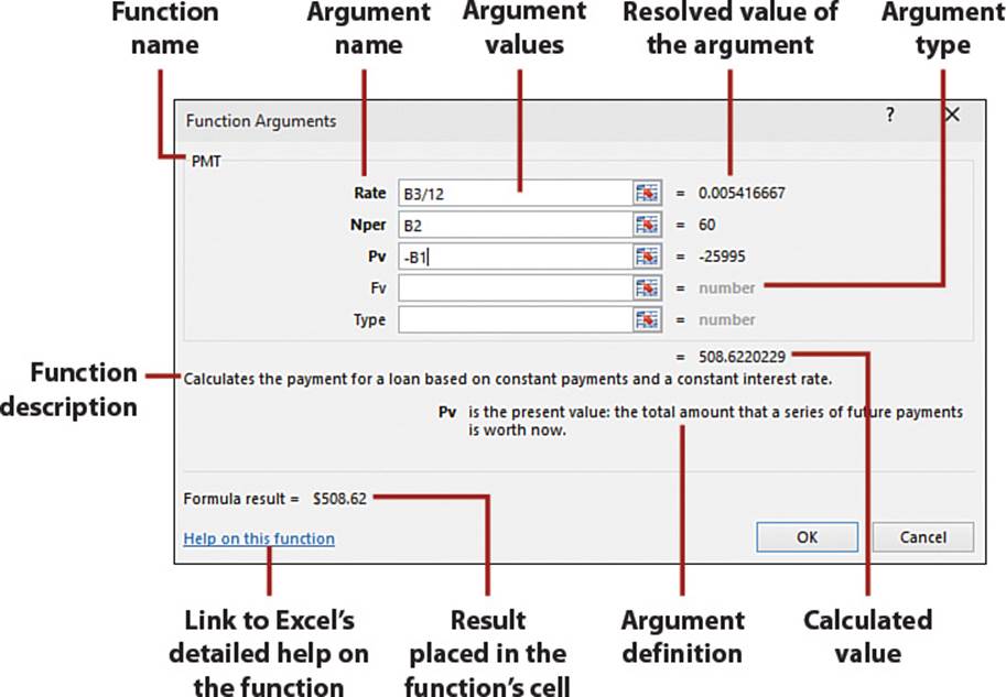
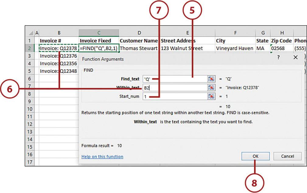
5. Select a field to enter an argument. Bold arguments are required; non-bold arguments are not. The argument type and description provide more information about the selected argument.
6. To select a range on a sheet, click in the field in the dialog box first; then select the range on the sheet.
7. To enter a value in the field, type it in. If the value is a word, wrap it in quotation marks; if the value is a number, don’t use quotation marks, or else the number will be treated as a word.
8. After you have filled in the required arguments, click OK to have the cell accept the function.
Enter Functions Using Formula Tips
If you are already familiar with the function you need, you can type it in the cell or formula bar directly.
1. Select the cell that will hold the formula.
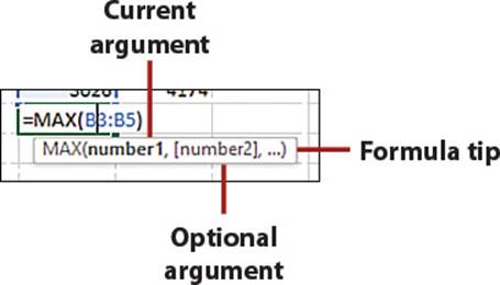
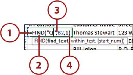
2. Type an equal sign (=), the function name, then a left parenthesis. The formula tip appears. The current argument is bold. Optional arguments appear in square brackets.
3. Use a comma to separate the arguments.
4. When you’re finished entering all the arguments, type the right parenthesis.
5. Press Enter or Tab to have the cell accept the formula.
Move the Formula Tip
If the formula tip is in the way, place your pointer on the tip where you can get a four-headed arrow then click and drag it out of your way.
Using the AutoSum Button
Excel provides one-click access to the SUM function through the AutoSum button. With two clicks, you can access a few more functions. In both cases, Excel will guess which cells you are trying to calculate and select them for you.
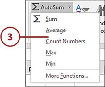
The functions available from the AutoSum button are as follows:
• Sum—Adds the values in the selected range by default
• Average—Averages the values in the selected range
• Count Numbers—Returns the number of cells containing numbers
• Max—Returns the largest value in the selected range
• Min—Returns the smallest value in the selected range
Calculate a Single Range
Use the AutoSum button to quickly calculate a range.
1. Select the range to sum, including the cell in which the formula will be placed.
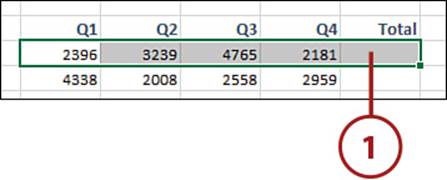
Skip the Range
You don’t have to pre-select the range you want to calculate. Instead, select only the cell where you want to place the formula. Excel will then try to figure out the range for you. You can accept it or select the one you want.
2. On the Home tab, click the AutoSum button.
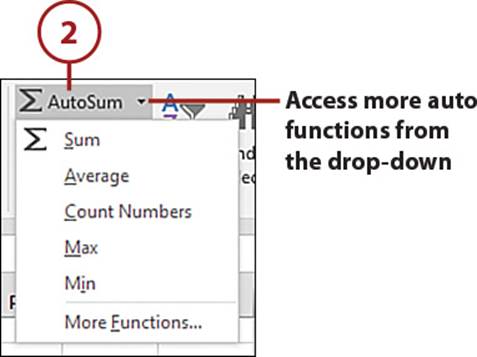
Apply Other Auto Functions
From the AutoSum drop-down, you can select another function, such as Average, to apply to the range.
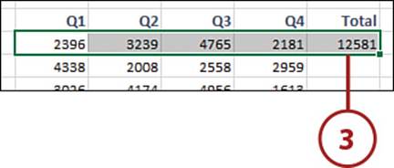
3. The formula is placed in the blank cell that is the far-right or bottom cell of the selection, and the value is calculated.
It’s Not All Good: Excel Misassumptions
You should keep an eye out for a couple of things when using the AutoSum function:
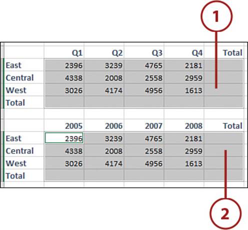
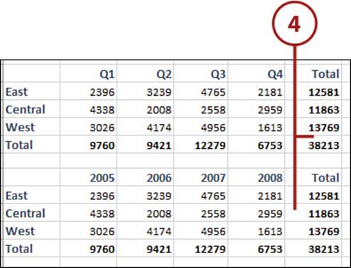
• Be careful of numeric headers (such as years) when letting Excel select the range for you. Excel cannot tell that the header isn’t part of the calculation range, and you will need to correct the selection before accepting the formula.
• Excel will look for a column to sum before summing a row. The default selection by Excel is the range of numbers above the selected cell, instead of the adjacent row of numbers.
Sum Rows and Columns at the Same Time
You can sum multiple, nonadjacent ranges at the same time.
1. Select the range to sum, including an extra row and column for the formulas.
2. While holding down the Ctrl key, select the other range with additional cells for the formulas.
3. Click the AutoSum button, or select an option from its drop-down.
4. Excel will enter the formulas in the extra cells.
Quick Calculations
You can use the status bar or the Quick Analysis icon to perform quick calculations with functions.
Calculate Results Quickly
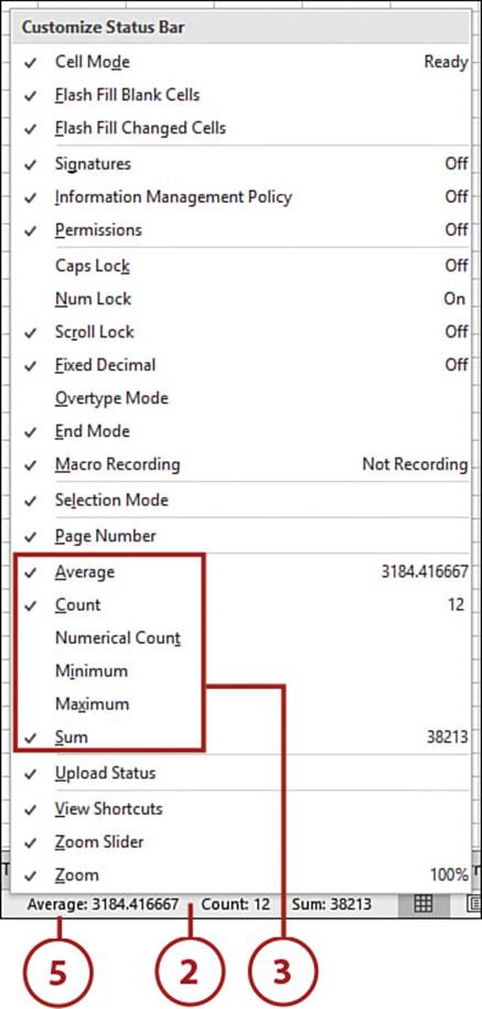
If you just need to see the results of a calculation and not include the information on a sheet, Excel offers six quick calculations you can preview in the status bar.
Changing the Status Bar
Changes to the status bar affect the application, not just the active workbook or sheet.
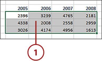
1. Select the range to calculate.
2. Right-click the status bar.
3. Select the functions you want to view or remove in the status bar.
4. Click away from the menu to return to Excel.
5. The selected results will appear in the status bar.
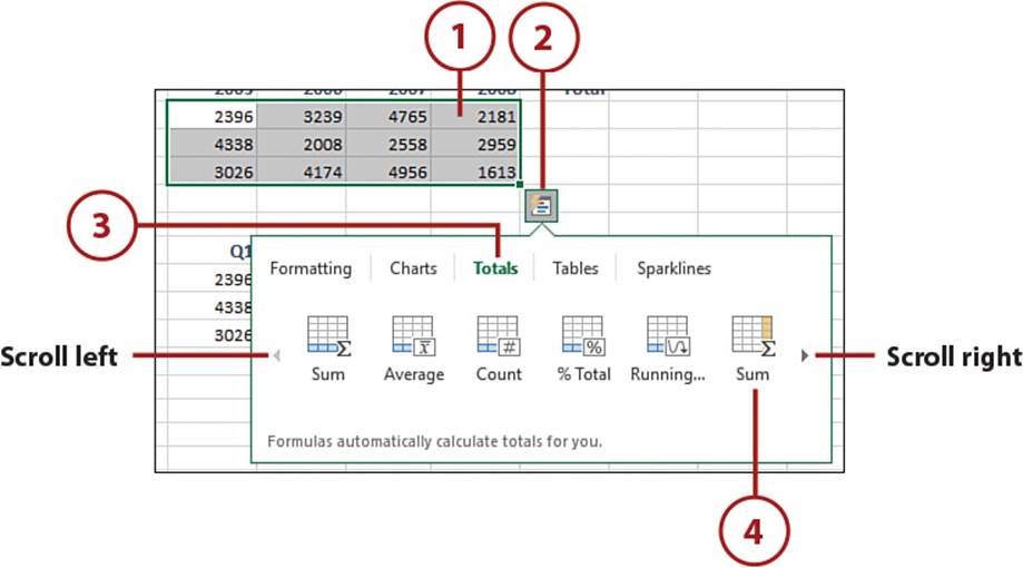
Using Quick Analysis Functions
When you select multiple adjacent cells, the Quick Analysis icon appears in the bottom-right corner of the selection. Click the icon, select TOTALS, and various quick calculations will appear.
1. Select the range to calculate.
2. Click the Quick Analysis Icon.
3. Select Totals.
4. Choose the desired function. Use the arrows on the left and right sides of the icons to scroll through the list.
Using Lookup Functions
This section reviews some of the lookup functions. There are functions that can return a value dependent on its position in a list or return a value in the same row as a match. You can even combine multiple functions to return a value by looking up and matching multiple variables.
Use CHOOSE to Return the nth Value from a List
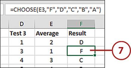
The CHOOSE function returns a value from the list based on an index number. The syntax of the CHOOSE function is as follows:
CHOOSE(index_num, value1, [value2],...)
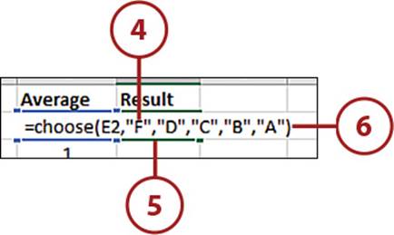
In the following example, the numeric grade is used as the index number, and a letter grade is supplied based on its position in the list. For example, if the numeric grade is “1,” the letter in the first position, “F,” is returned.
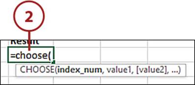
1. Select the cell for the formula.
2. Type the following:
=CHOOSE(
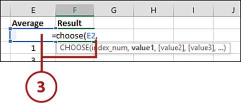
3. Select the cell with the index number and then type a comma.
4. Select the cell with the first value argument, or type it in. If it’s an alphabetic character, wrap it in quotation marks.
5. Type a comma then enter the next value. Repeat until all the values are entered.
6. Type the closing parentheses and press Enter or Tab.
7. Based on the index number, Excel will return the corresponding value.
Function Rules
Here are a few rules to keep in mind when using CHOOSE:
• If the index_num is a decimal, it will be rounded to the next lowest integer. For example, if it is 4.8, the formula will use 4.
• If the index_num is less than 1 or greater than the number of available values, the function will return a #VALUE! error.
• You can enter 1 to 254 argument values.
• Arguments can be numbers, cell references, names, formulas, functions, or text.
Use VLOOKUP to Return a Value from a Table
The VLOOKUP function matches your lookup value to a value in a dataset and returns data from a specified column in the matching row. For example, based on a customer’s name, you can use VLOOKUP to fill in the street address and phone number. The syntax of the VLOOKUP function is as follows:
VLOOKUP(lookup_value, table_array, col_index_num, [range_lookup])
1. Select the cell for the formula.
2. Type =VLOOKUP( and then press the fx button by the formula bar.
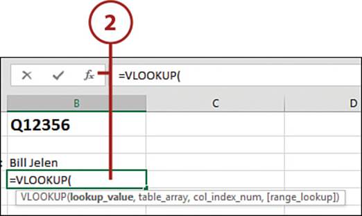
3. Select the cell with the value to look up. Press F4 to change the cell address from relative to absolute. That way, when you copy the formula, the Lookup_value address won’t change.
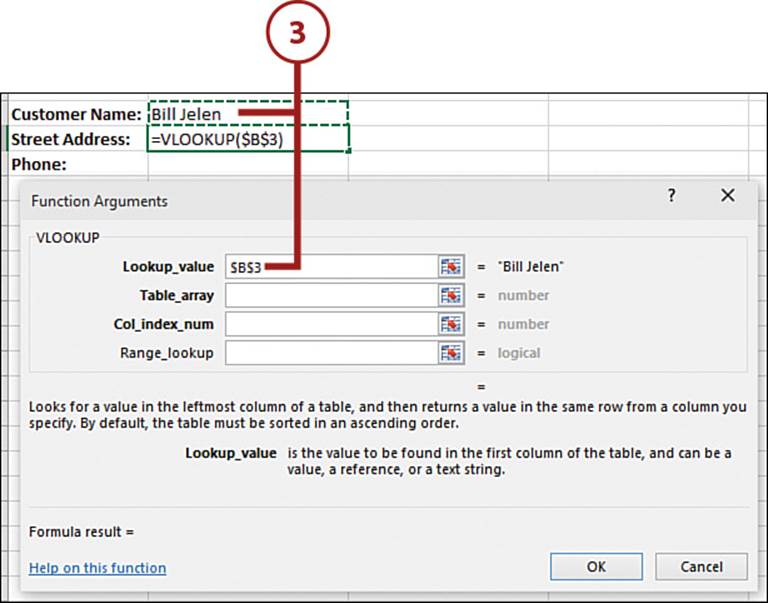
4. Click in the Table_array field and then select the lookup range, ensuring that the lookup value is in the leftmost column of the selection. Press F4 to change the cell address from relative to absolute.

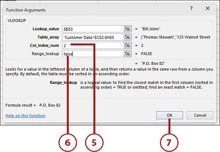
5. Enter the index number of the column to return in the Col_index_num field. This is based on the lookup range and may not be equivalent to the column heading. For example, if the selected range begins in column C and the col_index_num is 2, a value from column D will be returned.
6. Enter False if you want to return an exact match to the lookup value.
7. Click OK to complete the function.
>>>Go Further: Troubleshoot VLOOKUP Errors
If VLOOKUP returns an error or incorrect value but you can manually verify that the lookup value is present in the table, the issue may be one of the following:
• If you’re using FALSE for the range_lookup, the entire cell contents must match 100%. If you’re looking up “Bracelet” and the term in the table is “Bracelets,” Excel will not return a match.
• Be careful of extra spaces before and after a word. “Bracelet” and “Bracelet” are not matches—the first occurrence has a space at the end.
• If you’re matching numbers, make sure both the lookup value and the matching value are formatted the same type—for example, both as General or one as General and the other as Currency. This allows Excel to still see them as numbers. Sometimes when you’re importing data, numbers get formatted as Text. If you have a lookup value formatted as General and the matching value is formatted as Text, Excel will not see this as a match. Refer to the section “Fixing Numbers Stored as Text” in Chapter 4, “Getting Data onto a Sheet,” for instructions on how to force the numbers stored as text to become true numbers.
• Make sure the table_array encompasses the entire dataset.
Use INDEX and MATCH to Return a Value from the Left
VLOOKUP works only when returning data from columns to the right of the lookup column. If your data is also to the left of the lookup column, use MATCH and INDEX together. The INDEX function returns a value based on a row and column number. The MATCH function looks up a value and returns its position (row or column) in a dataset.
The syntax of the INDEX function is as follows:
INDEX(array, row_num, [column_num])
Two Ways to Use INDEX
The INDEX function has two syntaxes—array and reference—but this section will only use the array version.
And here is the syntax of the MATCH function:
MATCH(lookup_value, lookup_array, [match_type])
1. Select the cell for the formula.
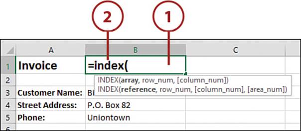
2. Type the following:
=INDEX(
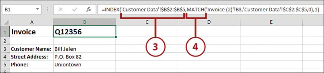
3. Select the range you want to return data from, press F4 to make the address absolute, and then type a comma.
4. The next argument for the INDEX function is the row_num. Because this is our dynamic value, use the MATCH function to do the lookup and return the row number. Type the following:
MATCH(
Switching Sheets When Writing Formulas
Sometimes when writing formulas, you have to switch to another sheet to select a range. When you switch back to the sheet you are entering the formula on, Excel includes the sheet name in the formula. It’s up to you whether or not you want to keep this unneeded reference.
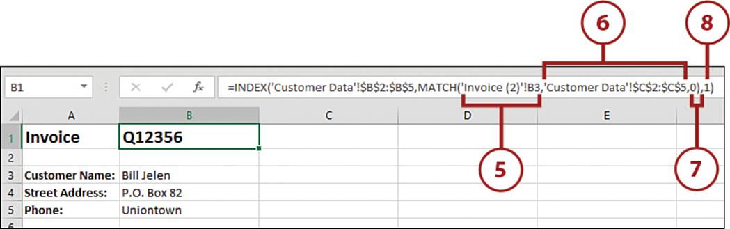
5. Select the lookup value and then type a comma.
6. Select the lookup range and then type a comma.
7. Enter the match type. The MATCH function is now complete, so type the following:
),
• If the match type is 1, the function returns the largest value that is less than or equal to the lookup_value. The lookup_array must be sorted in ascending order.
• If 0, the function returns the first value that is an exact match to the lookup_value.
• If -1, the function returns the smallest value that is greater than or equal to the lookup_value. The lookup_array must be sorted in descending order.
8. Enter the index number of the column to return. This is based on the lookup range and may not be equivalent to the column heading. For example, if the table begins in column B and the col_index_num is 2, a value from column C will be returned.
9. Enter the closing parenthesis and press Enter or Tab to calculate the formula.
Nested Functions
It’s not always easy to type in a formula that uses multiple functions. You may find it easier to place each function in a different cell, referencing the results of a previous function as needed. When you’ve verified that each piece works, cut the function (without the equal sign) out of its cell and paste it over the cell address in the parent function.
Using SUMIFS to Sum Based on Multiple Criteria
The SUMIFS function sums a single column based on multiple criteria. For example, you can sum revenue between two dates or sum the quantity of a specific product in a specific region.
Here is the syntax of the function (optional arguments are in square brackets):
SUMIFS(sum_range, criteria_range1, criteria1, [criteria_range2, criteria2],...)
SUMIFS Rules
You need to keep a few rules in mind when using this function:
• Each range consists of a single column.
• Each range has the same number of rows.
• Words as well as equality and inequality symbols must be wrapped in quotation marks.
• If you are using equality and inequality symbols with a cell reference, the cell reference should be outside the quotation marks around the symbol. Also, join the symbols and cell reference with an ampersand (&).
Sum a Column Based on Two Criteria
The following example sums the revenue of records within a specific date range with a maximum quantity.
1. Select the cell for the formula.
2. Type the following:
=SUMIFS(
3. Click the fx button by the formula bar.
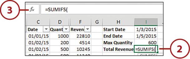
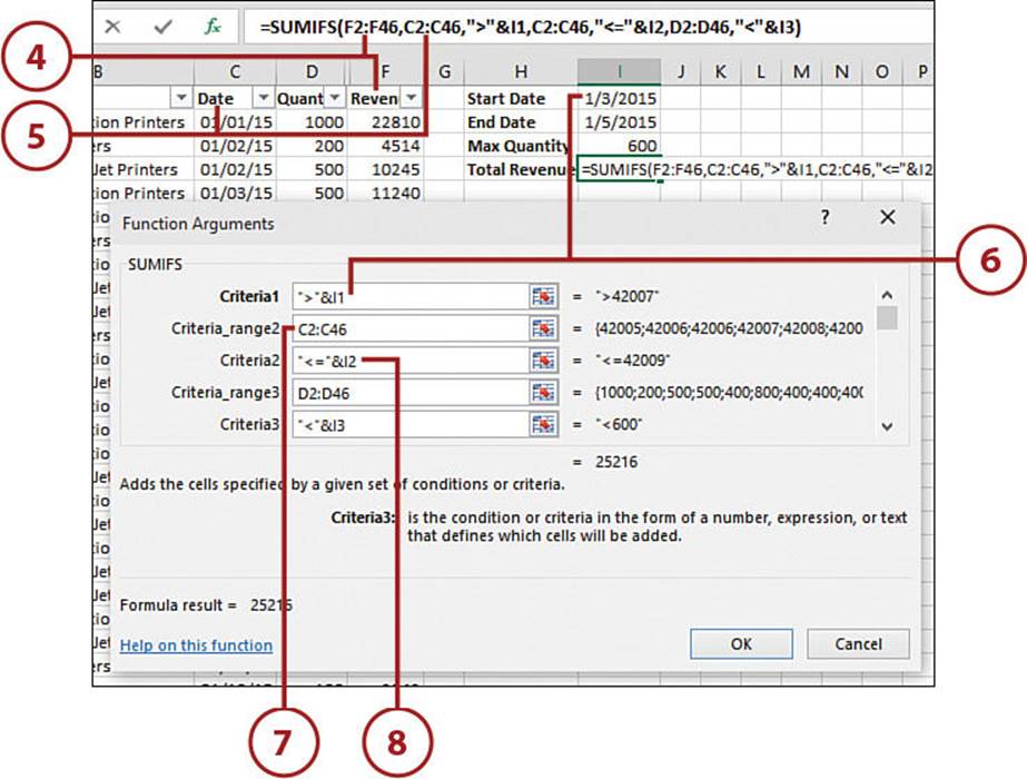
4. Select the range to sum (in this case, Revenue).
5. Click in the Criteria_range1 field and select the first criteria range, Date. Notice that when you click in the field, more fields are added to the dialog box.
6. The first criteria is dates greater than the start date. Click in the Criteria1 field and type the following:
“>”&
Then select the cell with the start date.
7. Click in the Criteria_range2 field and select the second criteria range, which again is the Date column.
8. The second criteria is dates less than or equal to the end date. Click in the Criteria2 field and type the following:
“<=”&
Then select the cell with the end date.
View More Fields
As fields are filled in, more are added, but the dialog box doesn’t get bigger. Use the scroll bar on the right side of the dialog box to scroll down to the next field as needed.
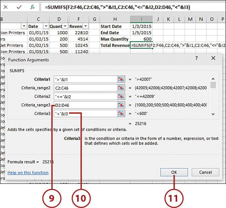
9. Click the in the Criteria_range3 field and select the third criteria range, the Quantity column.
10. The third criteria is quantities less than a set maximum. Click in the Criteria3 field and type the following:
“<”&
Then select the cell with the max quantity.
11. Click OK to have Excel accept the formula and calculate it.
12. Change the dates and max quantity and watch the total revenue update.
Using IF Statements
The IF function lets you build a statement where you perform a logical test, such as comparing two values, and then do one thing if the test evaluates to TRUE and another if it’s FALSE. The function syntax is as follows:
IF(logical_test, [value_if_true], [value_if_false])
Compare Two Values
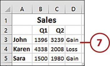
The following example compares the quarter sales for each salesperson. If sales have gone up, “Gain” is entered in the cell; otherwise, “Loss” is entered.
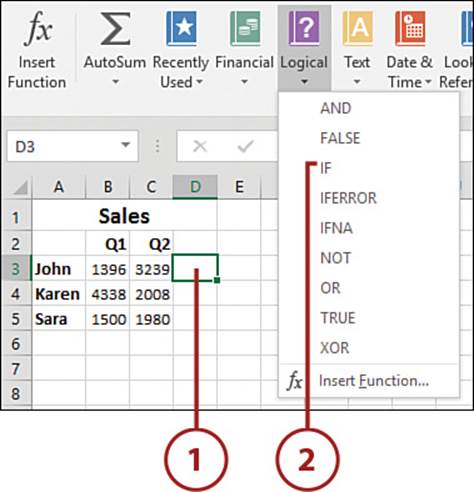
1. Select the cell where the formula will go.
2. Select IF from the Logical drop-down on the Formulas tab.
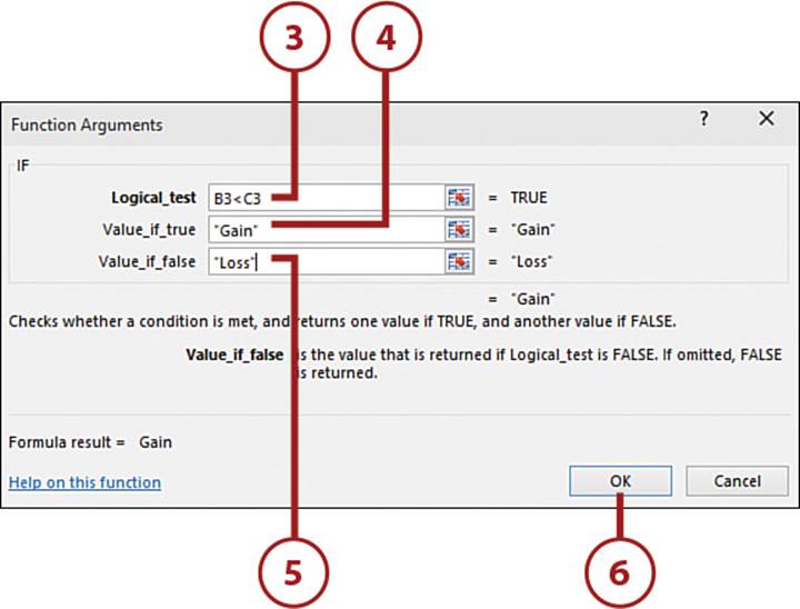
3. The Logical_test field is where we enter our values to compare. Select the cell containing the first value to compare, enter the comparison symbol < (less than), and then select the cell containing the second value to compare.
4. In the Value_if_True field, type “Gain”.
5. In the Value_if_False field, type “Loss”.
6. Click OK. Excel will calculate the formula result.
7. Copy the formula to other cells in the dataset.
>>>Go Further: Combine IF with Other Logical Functions
You can combine the IF statement with AND, OR, and NOT to expand the logical test.
• AND—Returns TRUE if all its arguments are TRUE. Returns FALSE if any of the arguments evaluate to FALSE. The function syntax is
AND(logical1, [logical2], ...)
• OR—Returns TRUE if any of its arguments are TRUE. Returns FALSE if all the arguments evaluate to FALSE. The function syntax is
OR(logical1, [logical2, ...])
• NOT—Reverses the logic of its arguments. The function syntax is
NOT(logical)
For example, to check if a value in cell B3 is between 2000 and 6000, use AND like this:
=IF(AND(B3>2000,B3<6000),”Between”, “Not Between”)
To check that the value is not between those numbers, you could do this:
=IF(NOT(AND(B3>2000,B3<6000)),”Not Between”, “Between”)
Hiding Errors with IFERROR
The IFERROR function returns the value specified if a formula evaluates to an error; otherwise, it returns the result of the formula. The function syntax is as follows:
IFERROR(value, value_if_error)
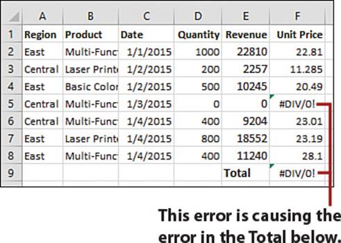
Hide a #DIV/0! Error
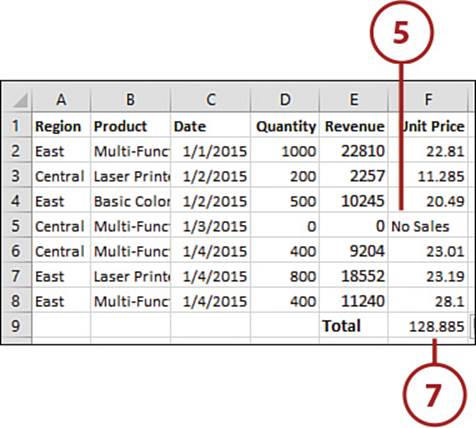
If there’s an error in a column being summed, the sum will also be an error. Wrap the calculation that produces the first error in an IFERROR so the sum formula will calculate properly.
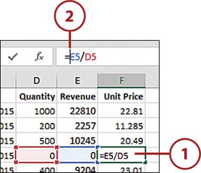
1. Select the cell with the formula producing the #DIV/0! error.
2. Place your cursor after the equal sign (=) in the formula bar.
3. Type IFERROR( and then place your cursor at the end of the formula.
4. Type a comma and then “No Sales”) (or some other value).
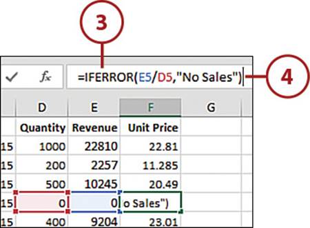
5. Press Enter or Tab to have Excel accept and calculate the formula.
6. Copy the formula to the rest of the range.
7. The sum formula no longer calculates to an error.
Understanding Dates and Times
Understanding how Excel stores dates and times is important so that you can successfully use formulas and functions when calculating with dates and times.
Dates and times in Excel are not stored the same way we see them. For example, you may type 9/8/15 into a cell, but Excel actually sees 42255. That number, 42255, is called a date serial number. The formatted value, 9/8/15, is called a date value. Storing dates and times as serial numbers allows Excel to do date and time calculations.
Time serial numbers are stored as decimals, starting at 0.0 for 12:00 a.m. and ending at 0.9999884259 for 11:59:59 p.m. The rest of the day’s decimal values are equivalent to their calculated percentage, based on the number of hours in a day, 24. For example, 1:00 a.m. is 1/24 or .04166, and 6:00 p.m. would be the 18th hour of the day, 18/24 = 0.75.
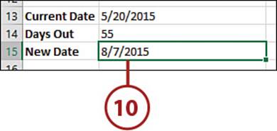
Return a New Date X Workdays from Date
Excel has a function called WORKDAY that returns a date before or after a specified number of workdays. You also have the option of specifying holidays to skip when calculating the new date.
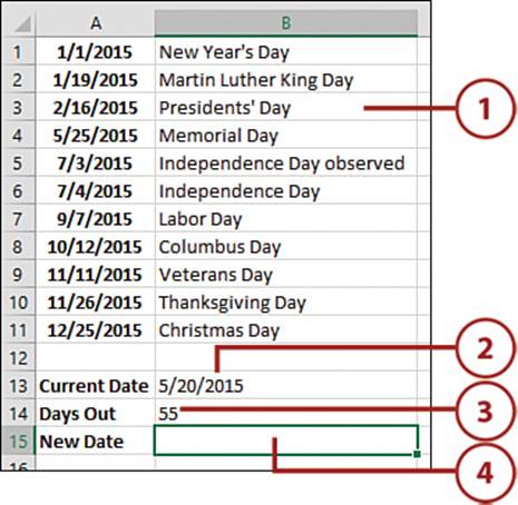
1. If you want to use the holidays argument, create a list of dates you want the calculation to skip when counting days.
2. Enter the starting date in a cell.
3. Enter the number of days out you want to count.
4. Select the cell for the formula.
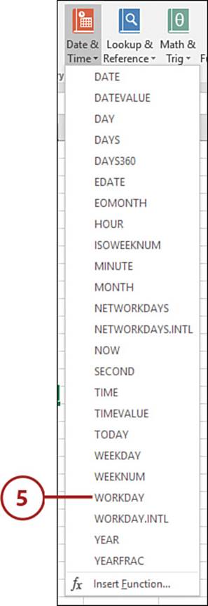
5. Select WORKDAY from the Date & Time drop-down on the Formulas tab.
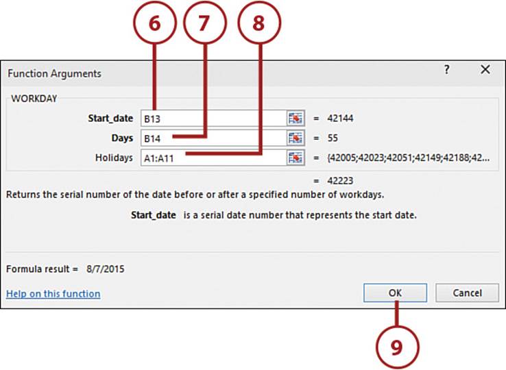
6. Select the cell with the start date.
7. Click in the Days field and then select the cell with the days to count.
8. Click in the Holidays field then select the range of holidays.
9. Click OK. Excel will calculate a new date.
10. Apply a date format to the cell if needed.
Calculate the Number of Days Between Dates
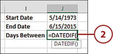
There’s a hidden function that can be used to calculate the days, months, or years between two dates. The function doesn’t appear when you look at a list of available date functions; Excel includes it for Lotus compatibility, but it can still be used, if you know how to get at it.
1. Select the cell for the formula.
2. Type the following:
=DATEDIF(
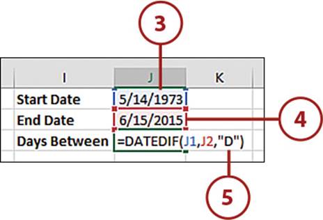
3. Select the cell with the oldest date and type a comma.
4. Select the cell with the newer date and type a comma.
5. Type the following:
“D”)
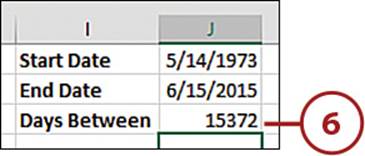
6. Press Enter or Tab to calculate the result.
>>>Go Further: More Third Argument Options
Six different options are available for the third argument, providing different ways of counting the time between the dates:
• “D”—The number of days between the dates
• “M”—The number of months between the dates
• “Y”—The number of years between the dates
• “YM”—The number of months between the dates, ignoring the days and years in the dates
• “YD”—The number of days between the dates, ignoring the years in the dates
• “MD”—The number of days between the dates, ignoring the months and years in the dates
Using Goal Seek
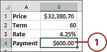
Goal Seek adjusts the value of a cell to get a specific result from another cell. For example, if you have the price, term, and rate of a loan, you can use the PMT function to calculate the payment. But what if the calculated payment wasn’t satisfactory and you wanted to recalculate with additional prices? You could take the time to enter a variety of prices, recalculating the payment. Alternatively, you could use Goal Seek to tell Excel what you want the payment to be and let it calculate the price for you.
Calculate the Best Payment
Here are a couple things to keep in mind when using Goal Seek:
• You must have the formula in the Set cell. Goal Seek works by plugging values in to your existing formula.
• A clear mathematical relationship between the starting and ending cells must exist.
1. Select the cell whose value you want to be a specific value.
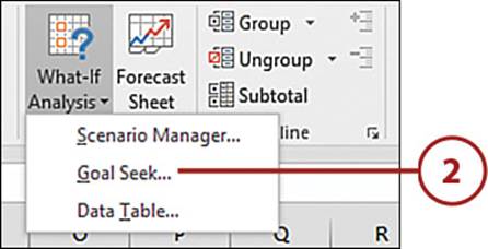
2. Select Goal Seek from the What-If Analysis drop-down on the Data tab.
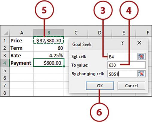
3. In the Set Cell field should be the address of the cell selected in step 1. If not, select the cell for which you are seeking a value.
4. In the To Value field, enter the value you want the Set cell to be, such as 630.
5. In the By Changing Cell field, select the cell whose value you want Excel to change so the Set Cell field calculates to the desired value.
6. Click OK.
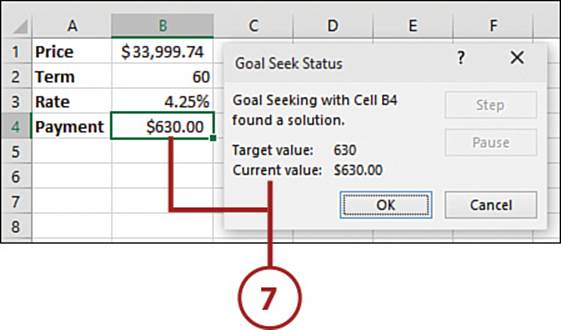
7. Excel will attempt to return a solution as close to the desired value as possible. If it succeeds, a message box will appear showing the target value and the actual value it attained.
Using the Function Arguments Dialog Box to Troubleshoot Formulas
If you have one function using other functions as arguments and the formula returns an error, you can use the Function Arguments dialog to track down which function is generating the error.
Narrow Down a Formula Error
The Function Arguments dialog box makes it easier to figure out which function in a multifunction formula is causing the problem.
1. Select the cell with the formula to troubleshoot.
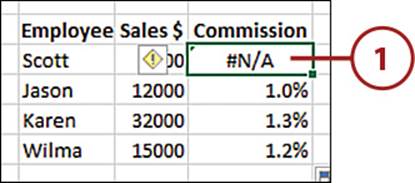
2. In the formula bar, place your cursor in the formula’s first function.
3. Click the fx button next to the formula bar.
4. If you see the error in the selected function, you can fix it and click OK to recalculate the formula. Otherwise, continue to the next step.
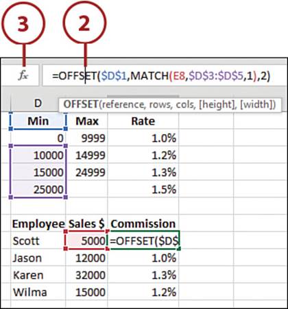
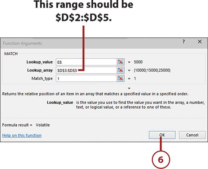
5. If you see the error in a field using another function, place your cursor in that function’s name in the formula bar.
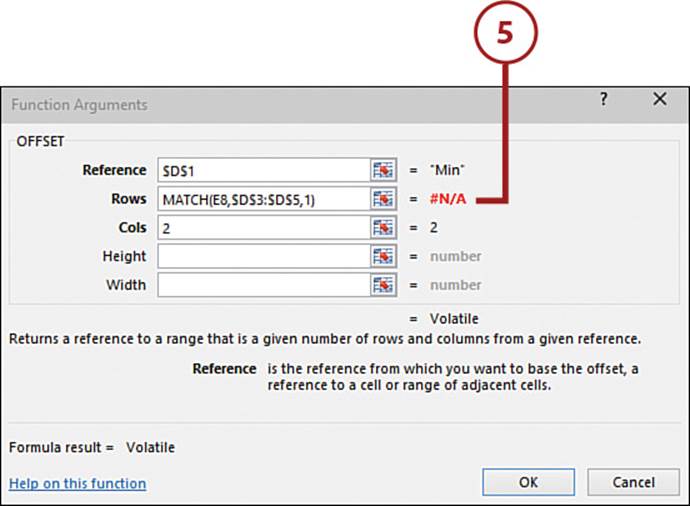
6. The selected function is loaded into the Function Arguments dialog box. Repeat this as needed to find which function is causing the error and fix it. Click OK when you are done.
All materials on the site are licensed Creative Commons Attribution-Sharealike 3.0 Unported CC BY-SA 3.0 & GNU Free Documentation License (GFDL)
If you are the copyright holder of any material contained on our site and intend to remove it, please contact our site administrator for approval.
© 2016-2026 All site design rights belong to S.Y.A.