Excel 2016 for Windows Pivot Tables (2016)
3. Grouping Items
Pivot tables let you combine items into groups, which you can use to subset related values that can’t be easily combined by sorting, filtering, or other means. Numbers, dates, times, and user-selected items can be grouped.
Grouping by Selected Items
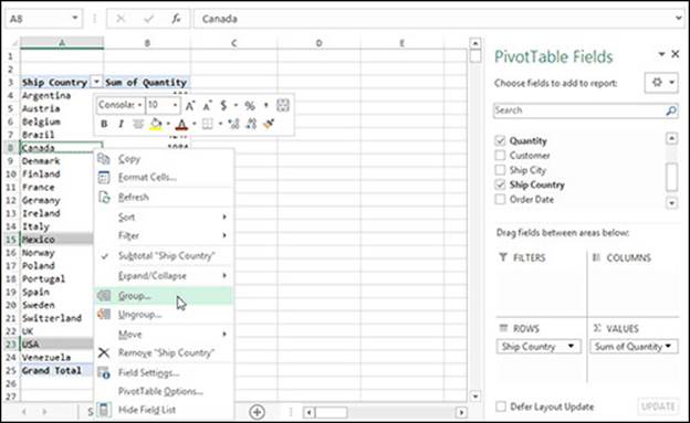
To create a custom group, select the items in the pivot table that you want to group, either by clicking or dragging, and then choose PivotTable Tools > Analyze tab > Group group > Group Selection (or right-click a selected cell and then choose Group from the shortcut menu).
Tip: To select adjacent cells, click the first cell and then Shift-click the last cell. To select nonadjacent cells, Ctrl-click each cell.
Consider a pivot table with the settings:
Rows: Ship Country
Columns: (empty)
Values: Quantity (summarized by Sum)
Filters: (empty)
In the pivot table, Ctrl-click Canada, Mexico, and USA; right-click any selected item; and then choose Group.
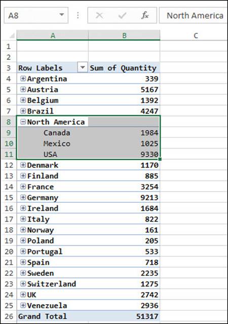
Replace the default group name (Group1) with a meaningful name (North America). Excel also creates a new virtual field named Ship Country2 in the Rows box, which you can pivot on (drag Ship Country2 to the Columns box, for example). To remove the grouping, right-click the group name and then choose Ungroup.
Nested Groups
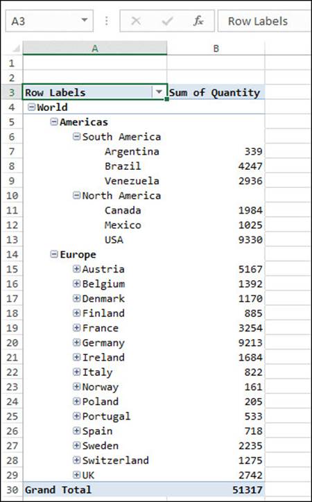
You can create any number of groups and even create nested groups (groups of groups). When you create nested groups, it’s usually easiest to define the broadest (outermost) group first and then progress to the innermost groups.
Grouping by Time Periods
When a field contains dates or times, you can create groups that summarize data by time periods (hours, months, years, and so on). You can use the Order Date field, for example, to summarize sales by month. Consider a pivot table with the settings:
Rows: Order Date
Columns: (empty)
Values: Quantity (summarized by Sum)
Filters: (empty)
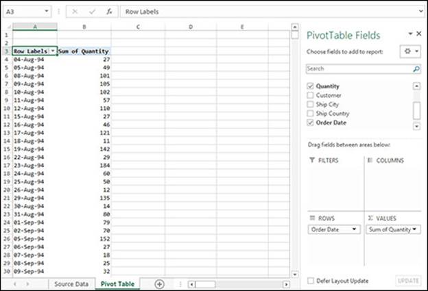
In the pivot table, right-click any cell in the Order Date (Rows) column and then select Group from the shortcut menu. The Grouping dialog box opens. In the By list, select Months and Years. Verify that the starting and ending dates are correct and then click OK.
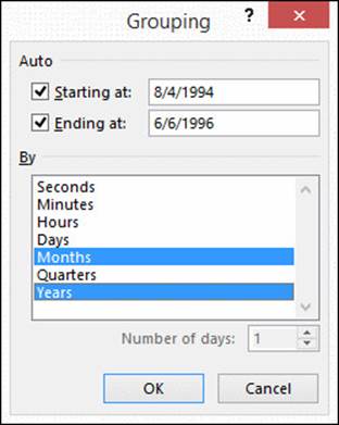
The Order Date items in the pivot table are grouped by years and by months. Excel also creates a new virtual field named Years in the Rows box, which you can pivot on (drag Years to the Columns box, for example). To remove the grouping, right-click any cell in the Order Date (Rows) column and then choose Ungroup.
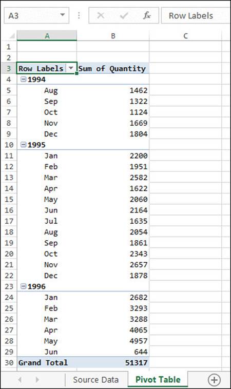
Tip: If you select only Months (and not Years) in the By list, then months in different years are combined. The Aug item, for example, would show the combined quantities for 1994 and 1995 (the data stop in June, 1996).
Grouping by Weeks
You can also group by week (or any fixed span of days). In the Grouping dialog box, select only Days (nothing else) in the By list and then type 7 in the “Number of days” box. Clear the “Starting at” checkbox and then adjust the start date to fall on the first day (typically, Sunday or Monday) of the first week of interest. If you like, adjust the end date too. Click OK.
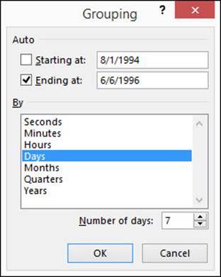
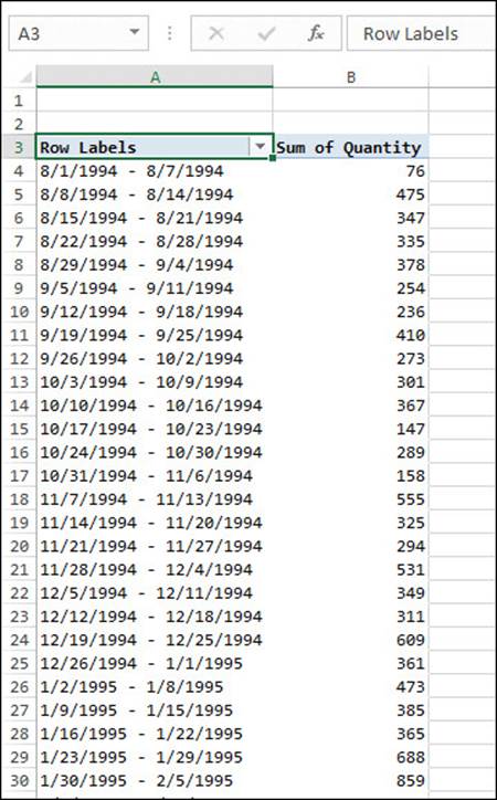
Each row in the resulting pivot table shows the start and end dates of each week.
Grouping by Numbers
You can group by numbers to create a frequency distribution, where each entry in the pivot table contains the frequency (count) of the occurrences of values within a particular group or interval. Consider a pivot table with the settings:
Rows: Quantity
Columns: (empty)
Values: Quantity (summarized by Sum)
Filters: (empty)
The pivot table shows the quantity of units sold and the corresponding number of orders. The goal is to determine how many quantities are in each 10-point range (1-10, 11-20, and so on).
In the pivot table, right-click any cell in the Quantity (Rows) column and then select Group from the shortcut menu.
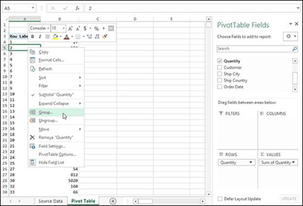
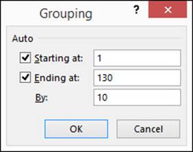
The Grouping dialog box opens. In the By box, type the size of the interval for each group (here, 10). Verify that the starting and ending points are correct and then click OK.
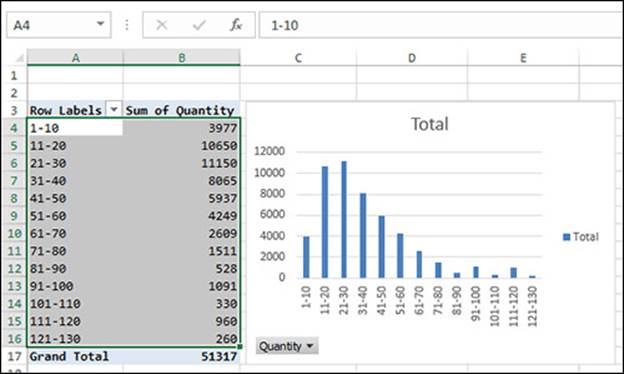
The Quantity items in the pivot table are grouped in uniform intervals (bins). The groups start at 1 and end at 130, in increments of 10. A column chart of a frequency distribution is a histogram ![]() . To remove the grouping, right-click any cell in the Quantity (Rows) column and then choose Ungroup.
. To remove the grouping, right-click any cell in the Quantity (Rows) column and then choose Ungroup.
Tip: By default, pivot tables don’t display items with a count of zero. To make sure that your frequency distribution has no gaps between intervals, select any cell in the interval column and then choose PivotTable Tools > Analyze tab > Active Field group > Field Settings > Layout & Print tab > select “Show items with no data”.
All materials on the site are licensed Creative Commons Attribution-Sharealike 3.0 Unported CC BY-SA 3.0 & GNU Free Documentation License (GFDL)
If you are the copyright holder of any material contained on our site and intend to remove it, please contact our site administrator for approval.
© 2016-2025 All site design rights belong to S.Y.A.