Excel 2016 for Windows Pivot Tables (2016)
4. Calculations and Custom Formulas
When you add a field to the Values box in the PivotTable Fields pane, Excel (in most cases) sums all the values in that field, but you can also calculate common statistics, do multiple calculations in the same pivot table, and create custom formulas.
Calculating Common Statistics
Excel’s preset calculations include common statistics: sum, count, average, maximum, percentage, rank, and so on.
To choose a preset calculation:
1. Select any cell in the pivot table.
Excel shows the PivotTable Fields pane.
2. In the PivotTable Fields pane, click the target field (“Sum of Quantity”, for example) in the Values box and then choose Value Field Settings from the pop-up menu.
The Value Field Settings dialog box opens.
3. In the “Summarize Values By” tab, choose a calculation in the list (Sum, Count, Average,...).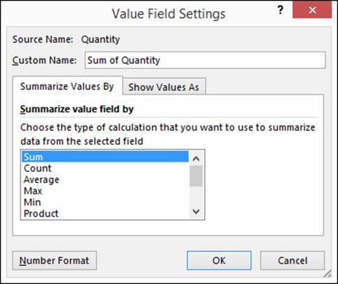
Alternatively, click the “Show Values As” tab to choose a more-complex calculation (percentage, difference, running total, rank, or index).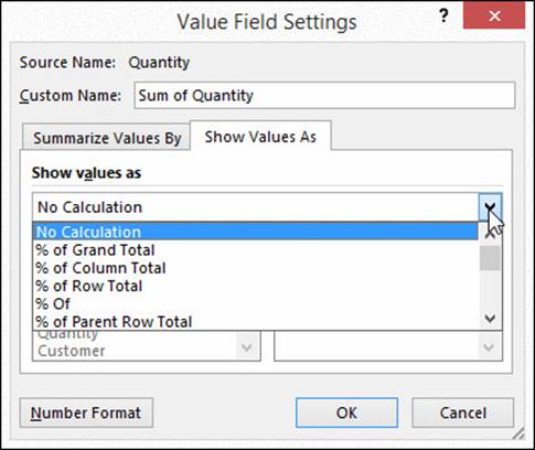
You can also change the default field name by typing a new name in the Custom Name box.
4. To format the field’s values, click Number Format, choose or define a new format, and then click OK.
You can change the number of decimal places, add a currency symbol, and so on.
5. Click OK to close the Value Field Settings dialog box.
Excel refreshes the pivot table with the new calculations.
Showing Zeros in Empty Cells
If the value of a pivot-table cell is zero, Excel shows it as an empty cell (inconsistent with non-pivot-table cells, which show zeros as zeros by default). To show zeros in a pivot table, right-click any cell in the pivot table and then choose PivotTable Options (or choose PivotTable Tools > Analyze tab > PivotTable group > Options). On the Layout & Format tab, clear the “For empty cells show” checkbox.
Calculating Multiple Statistics
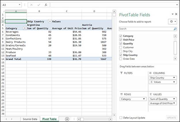
When you add multiple fields to the Values box, each field is calculated and shown in a separate column in the pivot table. To sum the Quantity and average the Unit Price, for example, drag both fields into the Values box and then follow the steps above to configure each field separately.
Similarly, you can do multiple calculations on the same field. To sum and average Quantity, for example, drag Quantity into the Values box twice and then configure the two Quantity fields separately.
Adding Custom Calculations
In addition to choosing a preset calculation, you can define a custom calculated field in a pivot table.
To add a calculated field:
1. Select any cell in the pivot table.
2. Choose PivotTable Tools > Analyze tab > Calculations group > Fields, Items, & Sets > Calculated Field.
The Insert Calculated Field dialog box opens.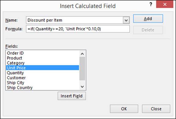
3. In the Name text box, type or paste a name for the new field.
4. In the Formula text box, enter the formula for this field.
The formula can use Excel’s built-in operators and functions, or change or combine one or more of the fields in the Fields list. To insert a field name in the formula quickly, double-click the name in the list. If you manually type a field name that contains spaces or special characters, enclose the name in single quotes ('Unit Price', for example).
5. Click OK.
In the PivotTable Fields pane, Excel adds the calculated field to the fields list and the Values box, so that it appears in the pivot table. Excel sums the formula for every row.
Removing a custom field from the Values box removes it from the pivot table, but it remains in the fields list for later use. To permanently delete a custom field, select it from the Name drop-down list in the Insert Calculated Field dialog box (shown above) and then click Delete.
Tip: To list all calculated fields in a new worksheet, choose PivotTable Tools > Analyze tab > Calculations group > Fields, Items, & Sets > List Formulas.
Troubleshooting Calculated Fields
Calculated fields have the following restrictions:
· A calculated-field formula can’t refer to pivot-table grand totals or subtotals, nor can it refer to worksheet cells by address or by name.
· You can summarize a calculated field by only Sum.
· Because calculated-field formulas are always applied against the sum of the underlying data, Excel calculates data fields, subtotals, and grand totals before evaluating the calculated field.
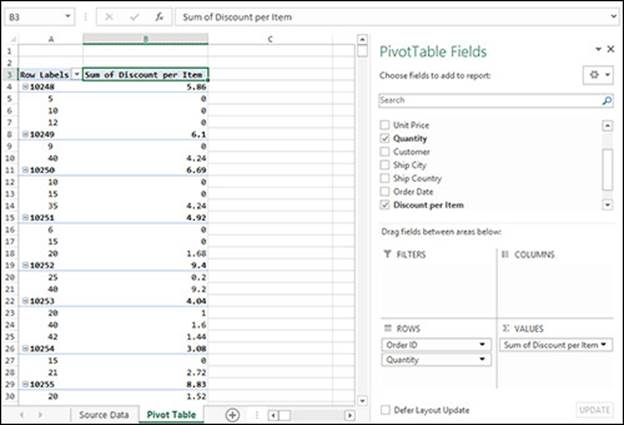
In nontrivial formulas, the last restriction can cause unexpected results because the sum of products (generally) isn’t equal to the product of sums. In the example above, the calculated field returns a 10 percent per-item price discount when a customer orders 20 or more units of a particular item, and no (zero) discount otherwise. In the resulting pivot table, the individual Quantity calculations are correct but the subtotals for each Order ID aren’t what you’d expect (because Excel sums all an order’s quantities before determining whether discounts apply). Another common trap: if you create a calculated field named Revenue with the formula:
='Unit Price' * Quantity
then Excel sums the prices, sums the quantities, and then multiplies the two sums—which is not what you want.
Sadly, there’s no way to fix this problem, but there are a few (somewhat unsatisfying) workarounds for when you want sum-of-products and Excel is giving you product-of-sums:
· Add a column (field) to the underlying source data. In the sample workbook, for example, you can add a revenue formula to column J in the Source Data worksheet: type Revenue in cell J1, type:
=D2*E2
in cell J2 (Unit Price × Quantity), and then fill down (Ctrl+D) the J2 formula to the end of the data (cell J2156).
· Copy (Ctrl+C) and paste values (Ctrl+Alt+V) from the pivot table to work with independently elsewhere in the workbook.
· Write formulas outside the pivot table. You might want to turn off the GETPIVOTDATA function when you write formulas that refer to a pivot table (PivotTable Tools > Analyze tab > PivotTable group > Options arrow > Generate GetPivotData toggle).
· Turn off grand totals and subtotals in the pivot table (PivotTable Tools > Design tab > Layout group) and then calculate your own totals outside the pivot table.
All materials on the site are licensed Creative Commons Attribution-Sharealike 3.0 Unported CC BY-SA 3.0 & GNU Free Documentation License (GFDL)
If you are the copyright holder of any material contained on our site and intend to remove it, please contact our site administrator for approval.
© 2016-2025 All site design rights belong to S.Y.A.