Excel 2016 for Windows Pivot Tables (2016)
5. Filtering Data
If a pivot table displays too much detail, you can filter (restrict) it to show only part of the source data. Excel offers several filters: report filters, slicers, and group filters.
Tip: If a pivot table’s data source is a table (Insert tab > Tables group > Table), then any filters that you apply directly to the table have no effect on linked pivot tables. To filter data from a pivot table, you must use one of the methods described in this chapter.
Report Filters
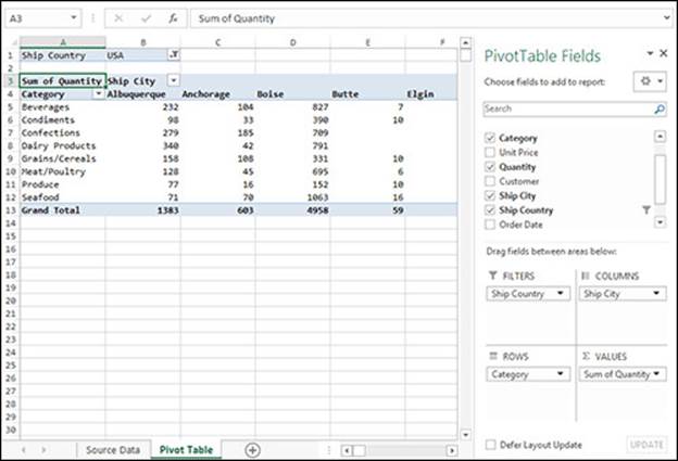
Report filters let you filter out data so that a pivot table uses only rows of interest in the source data. Start with a pivot table with the settings:
Rows: Category
Columns: Ship City
Values: Quantity (summarized by Sum)
Filters: (empty)
Now, to create a summary for only specific countries, drag the field Ship Country to the Filters box. The report filter field appears just above the pivot table. (If you use more than one report filter, each appears in a separate row.) To set the filter, click the drop-down arrow ![]() in the field box and then choose the countries that you want to display. To find an item, scroll the list or type the first few characters of its name in the search box. To filter for several items at the same time, turn on the Select Multiple Items checkbox and then select the desired items. When you’re done, click OK. When a filter is applied, the field box button changes to
in the field box and then choose the countries that you want to display. To find an item, scroll the list or type the first few characters of its name in the search box. To filter for several items at the same time, turn on the Select Multiple Items checkbox and then select the desired items. When you’re done, click OK. When a filter is applied, the field box button changes to ![]() and a filter (funnel) icon appears in the field list in the PivotTable Fields pane.
and a filter (funnel) icon appears in the field list in the PivotTable Fields pane.
Tip: To control how report filter fields are arranged in rows and columns, select any cell in the pivot table and then choose PivotTable Tools > Analyze tab > PivotTable group > Options > Layout & Format tab.
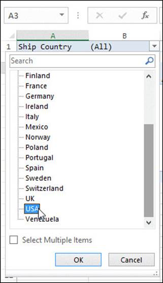
Excel uses checked items to create the pivot table, and ignores unchecked items. To quickly remove a report filter, choose the first item in the report filter list: “(All)”.
Tip: Any fields that you use for report filtering can’t also be used for grouping. If you filter by Ship Country, for example, you can’t also group by Ship Country. This restriction doesn’t apply to slicers and group filters.
Slicers
Slicers offer about the same features as report filters, but in “dashboard” format. Each slicer has its own floating window that you can format or drag around the main Excel window.
By contrast with report filters, slicers offer fast one-click filtering, and can filter and group on the same field. However, slicers tend to clutter your display with floating windows and don’t work well with fields that have many distinct values (which cause long scrolling distances). Also, slicers, like report filters, are less powerful than group filters.
To create a slicer:
1. Select any cell in the pivot table.
2. Choose PivotTable Tools > Analyze tab > Filter group > Insert Slicer.
The Insert Slicers dialog box opens, listing all the fields in the pivot table (except custom fields).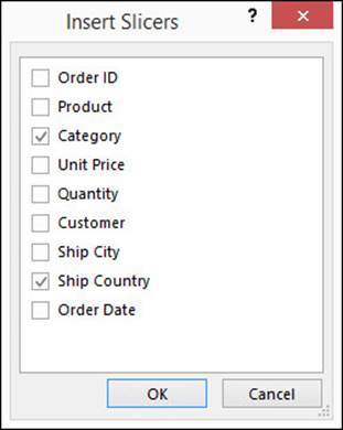 .
.
3. Select the checkbox of each field that you want to use for filtering.
Fields that have a small number of unique values make the best slicers because they fit well in a floating slicer window. Good choices: Category and Ship Country. Middling choices: Product and Customer. Poor choices: Unit Price and Order Date.
4. Click OK.
Excel adds a separate floating window for each slicer.
5. Move or resize the floating slicer windows as desired.
» To move a slicer, point to a border (the pointer turns into a four-way arrow) and then drag.
» To resize a slicer, point to a corner or the middle of an edge (the pointer turns into a two-way arrow) and then drag.
6. Use the slicer window to apply filtering. The slicer window lists all the unique values in a field, each value appearing as a separate button. The buttons of visible values are shaded. No filtering is in effect in a newly created slicer window, so every button is shaded.
» To filter on a single value, click its button.
» To filter on multiple values, click the ![]() toggle button at the top of the slicer window (or press Alt+S) and then click the desired filter buttons. Alternatively, hold down the Ctrl key while you click each button. (To select a range of contiguous values, click the first button and then Shift-click the last button.)
toggle button at the top of the slicer window (or press Alt+S) and then click the desired filter buttons. Alternatively, hold down the Ctrl key while you click each button. (To select a range of contiguous values, click the first button and then Shift-click the last button.)
» To clear filtering (show everything for the field), click the ![]() button at the top of the slicer window (or press Alt+C).
button at the top of the slicer window (or press Alt+C).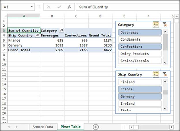
7. (Optional) Format the slicer.
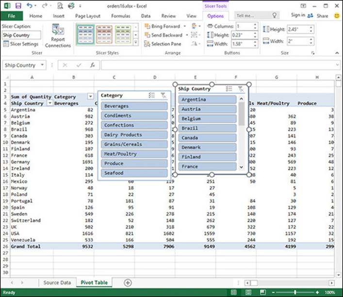
» To change the button colors, choose Slicer Tools > Options tab > Slicer Styles gallery.
» To expand or compact the slicer window, choose Slicer Tools > Options tab > Buttons group, and then change the Columns, Height, and Width values. The following figure shows a three-column slicer window with custom button colors.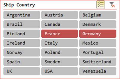
» To change the window title, choose Slicer Tools > Options tab > Slicer group > Slicer Caption box. To hide the window title, choose Slicer Tools > Options tab > Slicer group > Slicer Settings > clear “Display header”.
» To sort a slicer’s values, right click the slicer window and then choose a Sort command from the shortcut menu.
» To remove a slicer, click it and then press Delete (or right-click it and then choose the Remove command from the shortcut menu).
Timelines
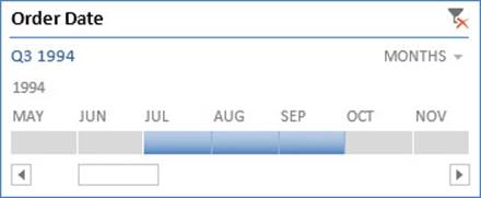
Timelines offer a visual way to view and change a contiguous range of dates and filter pivot tables and pivot charts. Timelines work like slicers. To create a timeline, select any cell in the pivot table and then choose PivotTable Tools > Analyze tab > Filter group > Insert Timeline. Drag or click the timeline controls to select time periods. To format the timeline, select (click) it and then choose Timeline Tools > Options tab.
Custom Slicer Styles
You can create custom slicer styles to reuse with as many slicers as you want.
To create a custom slicer style:
1. Choose Slicer Tools > Options tab > Slicer Styles group. Click the drop-down arrow ![]() and then choose New Slicer Style.
and then choose New Slicer Style.
The New Slicer Style dialog box opens.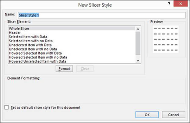
2. In the Name box, type a name for the new slicer style.
3. In the Slicer Element list, select an element.
Each element defines how a specific part of the slicer looks in a specific state. “Whole Slicer” formats the entire slicer and “Header” formats only the slicer’s window title. The specialized elements below “Header” format how an item looks when it’s selected, when it’s hovered over by the pointer, and when there’s no corresponding data for that value in the pivot table.
4. Click Format to format the selected element.
The Format Slicer Element dialog box opens. Change the font, border, and fill as desired and then click OK.
5. To format other elements in the slicer, repeat steps 3 and 4.
6. Click OK to create the style.
The custom style appears in the Slicer Styles gallery. You can apply it to any slicer, or right-click it to modify, delete, or duplicate it.
Group Filters
Group filters—more powerful than report filters and slicers—let you filter fields that you’re using to group a pivot table to:
· Show or hide specific items (like report filters, except that you can’t create report filters for grouping fields).
· Create complex conditions that subset data. You can show or hide dates that fall in a specific time period, for example, or names that begin or end with a certain letter.
· Filter on multiple fields and configure them independently (Excel additively applies every filter at the same time).
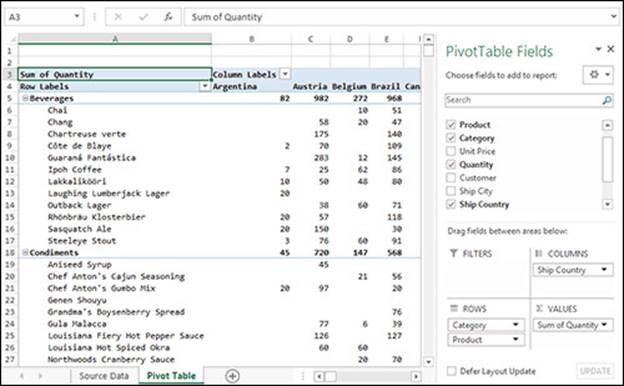
The examples in this section use a pivot table with the settings:
Rows: Category, Product
Columns: Ship Country
Values: Quantity (summarized by Sum)
Filters: (empty)
To create a group filter:
1. Click the drop-down arrow ![]() to the right of a Rows or Columns cell.
to the right of a Rows or Columns cell.
The filter list opens.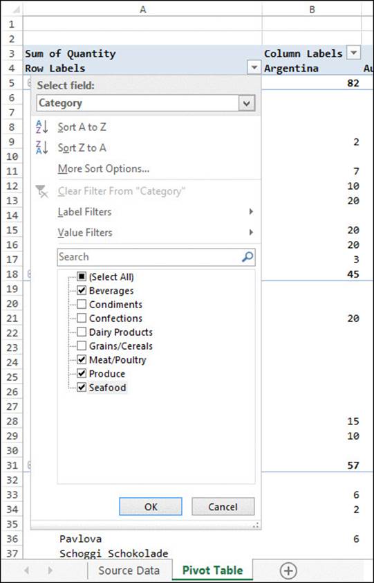
2. If you’re grouping on multiple fields, choose a field from the “Select field” drop-down list at top.
3. Set the desired options in the filter list and then click OK.
» To show or hide specific items, select or clear their checkboxes. To find an item, scroll the list or type the first few characters of its name in the search box.
» To show or hide items that contain specific text, begin or end with a certain letter, and so on, choose an option from the Label Filters submenu. To show only items that begin with “U”, for example, choose Label Filters > Begins With and then type U in the dialog box that opens.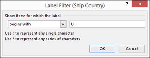
» To show or hide calculated values based on numerical criteria (less than, greater than, Top 10, and so on), choose an option from the Value Filters submenu. To show only items less than 500, for example, choose Value Filters > Less Than and then type 500 in the dialog box that opens.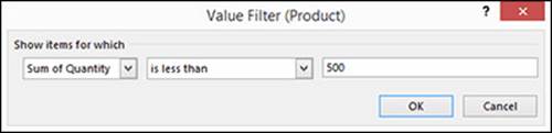
» To sort items in ascending, descending, or custom order, choose a Sort command.
» To remove a filter (show everything for the field), choose the Clear Filter command. If you have multiple filters, you must remove each one separately. To remove them all at once (and show all data), choose PivotTable Tools > Analyze tab > Actions group > Clear > Clear Filters.
Tip: When a filter is applied, the button to the right of the Rows or Columns cell changes to ![]() and a filter (funnel) icon appears in the field list in the PivotTable Fields pane.
and a filter (funnel) icon appears in the field list in the PivotTable Fields pane.
4. To filter by other grouping fields, repeat the preceding steps for each row label or column label.
Filtering Nested Fields
Label filters and value filters can get tricky when you work with nested fields. The effect of the Value Filters > Less Than > 500 command, for example, differs depending on whether you apply it to the Product or Category field (recall that Product is nested within Category in this example). Applied to Product, the pivot table shows products that sold fewer than 500 units (as you’d expect). Applied to Category, only categories with sales fewer than 500 units across all their products appear. Because every category has sales greater than 500 units in the current example, the filter hides every category and shows an empty pivot table (which is correct logically but might not be what you’d expect).
Note that if you apply a filter to a Rows field (Category or Products, in this example), your Columns fields (Ship Country) have no effect. Likewise, row filters don’t affect column filters.
All materials on the site are licensed Creative Commons Attribution-Sharealike 3.0 Unported CC BY-SA 3.0 & GNU Free Documentation License (GFDL)
If you are the copyright holder of any material contained on our site and intend to remove it, please contact our site administrator for approval.
© 2016-2025 All site design rights belong to S.Y.A.