Excel 2016 for Windows Pivot Tables (2016)

7. Tricks with Pivot Tables

Excel’s arsenal of pivot-table features offers a few nonobvious ways to solve common problems.

Creating a Frequency Tabulation

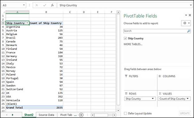
You can use a pivot table to quickly create a frequency tabulation for a single column of data. In the sample workbook, for example, switch to the Source Data worksheet, select the Ship Country column (click the H column heading), choose Insert tab > Tables group > PivotTable, and thencreate the pivot table. In the PivotTable Fields pane, drag the Ship Country field into the Rows box and then drag it again into the Values box. The resulting pivot table tallies the number of times that each country appears in the column. You can group, filter, and chart this tabulation as you would any pivot table. See also Grouping by Numbers.

Unlinking a Pivot Table from its Source Data

Excel doesn’t provide a direct way to “unlink” a pivot table from its source data, but you can create an unlinked copy of a pivot table in a few steps (handy if you want to send someone a pivot table summary report but not its underlying data).

To create an unlinked copy of a pivot table:

1. Select the entire pivot table.

To select the entire pivot table, drag to select all the pivot table’s cells. Or click anywhere in the pivot table and then choose PivotTable Tools > Analyze tab > Actions group > Select arrow > Entire PivotTable.

2. Press Ctrl+C (Home tab > Clipboard group > Copy).

3. Choose Home tab > Clipboard group > Paste arrow > Values.

Excel replaces the pivot table by its values, but without formatting.

4. In the Home tab > Clipboard group, click the tiny dialog box launcher icon in the bottom-right corner of the group.

The Clipboard pane opens.

5. In the Clipboard pane (with the unlinked pivot table still selected), click the item that corresponds to the pivot table copy operation. That is, the most-recent action (unless you did something else in Office after the copy).

Excel restores the original formatting in the unlinked pivot table. You can close the Clipboard pane.

Converting a Summary Table to a List

If you have a two-dimensional summary table (an ordinary range of cells—not a pivot table), you can reverse the usual pivot-table procedure by converting the summary table to a list. Data in list form can be easier to sort, filter, and update than data in summary form.

To convert a summary to a list, you must first add the PivotTable and PivotChart Wizard command to your Quick Access toolbar. Excel still supports this wizard, but it’s hidden by default.

To access the PivotTable and PivotChart wizard:

1. Right-click the Quick Access toolbar (at the top-left corner of the Excel window) and then choose Customize Quick Access Toolbar from the shortcut menu.

The Excel Options dialog box opens to the Quick Access Toolbar tab.

2. In the “Choose commands from” drop-down list, choose “Commands Not in the Ribbon”.

3. Scroll down the list (on the left) and then select PivotTable and PivotChart Wizard.

4. Click Add.

5. Click OK.

The PivotTable and PivotChart Wizard icon appears in the Quick Access toolbar.

The following example works for the specific summary table shown below, but you can easily modify the steps to work with your data.

To convert a summary table to a list:

1. Select any cell in the summary table.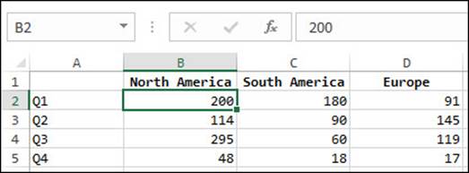

2. In the Quick Access toolbar, click the PivotTable and PivotChart Wizard icon .

The PivotTable and PivotChart Wizard dialog box opens.

3. Select “Multiple consolidation ranges” and then click Next.

4. Select “I will create the page fields” and then click Next.

5. Specify the range of the summary table in the Range box (here, A1:D5), click Add, and then click Next.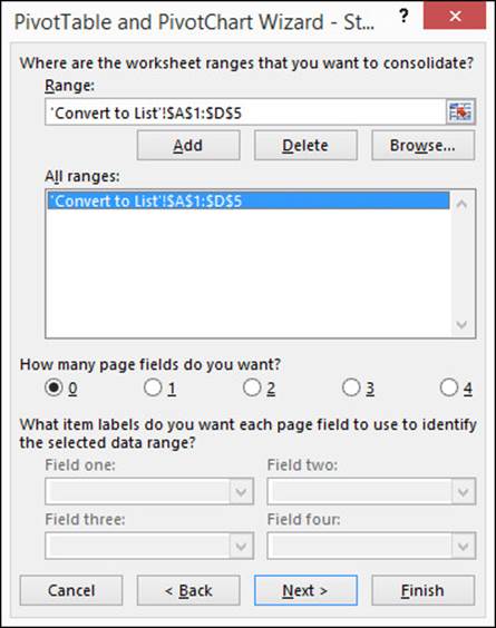

6. Specify a target location for the pivot table and then click Finish.

Excel creates a pivot table from the summary table and shows the PivotTable Fields pane.

7. In the PivotTable Fields pane, clear the checkboxes for the fields named Row and Column.

The pivot table shows a single field (Sum of Value), containing the sum of all the values in the table.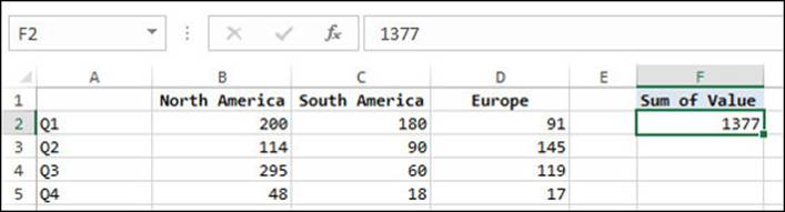

8. Double-click the cell that contains the total.

Excel creates a new worksheet that shows the original summary data in list form. Every value in the original summary table is converted to a row, which also contains the value’s corresponding row and column labels. You can change the default column headings (Row, Column, and Value) to meaningful names.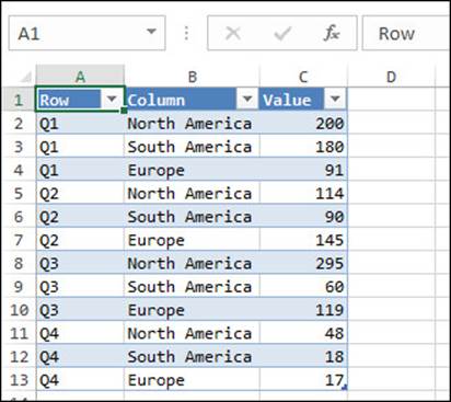

Controlling References to Pivot Table Cells

If you create a formula that refers to a cell within a pivot table, Excel automatically converts the cell reference to a GETPIVOTDATA function with arguments. For example:

=GETPIVOTDATA("Quantity", $A$3, "Category", "Beverages", "Ship Country", "Argentina")

GETPIVOTDATA ensures that formulas still return the correct results even if you rearrange the pivot table. To avoid GETPIVOTDATA autoconversion, don’t point to (click) the cell when you create the formula; instead, type the cell reference manually. To turn on or off GETPIVOTDATA autoconversion, choose PivotTable Tools > Analyze tab > PivotTable group > Options arrow > Generate GetPivotData toggle. Alternatively, choose File tab > Options > Formulas (on the left) > “Use GetPivotData functions for PivotTable references” checkbox.

Replicating a Pivot Table for Report Filter Items

You can set up a pivot table and then replicate it for every distinct value of a report filter. This feature isn’t popular because it generates multiple pivot tables when a single nested and filtered pivot table should suffice for most purposes. It may be useful for generating separate tables or charts to paste in different slides in a presentation. Consider a pivot table with the settings:

Rows: Category
Columns: (empty)
Values: Quantity (summarized by Sum)
Filters: Ship Country

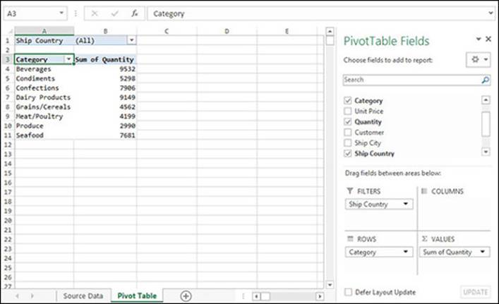
Choose PivotTable Tools > Analyze tab > PivotTable group > Options arrow > Show Report Filter Pages command. In the Show Report Filter Pages dialog box that opens, select Ship Country and then click OK. Excel replicates the pivot table for every country, creating a worksheet for each new pivot table (inspect the worksheet tabs at the bottom of the Excel window).

Sorting a Pivot Table Manually

You can sort the rows or columns of a pivot table automatically by clicking the drop-down arrow to the right of a Rows or Columns cell, or sort them manually by dragging.

To sort a pivot table manually:

1. In the pivot table, right-click any row or column label of the field that you want to sort and then choose Sort > More Sort Options > Manual > OK.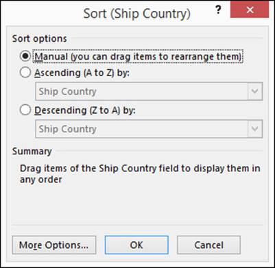

2. Select the label cell of the row or column that you want to move. If you want to move a group of adjacent rows or columns, drag to select multiple label cells.

3. Hover the pointer over the border of the selected label cell(s) until the pointer changes to a four-way arrow (called a move pointer). You may have to move the pointer slowly around the border until it changes to a move pointer.

4. Drag the selected row(s) or column(s) to another location within the pivot table.

As you drag, a thin line appears to show where the selection will land when dropped.