Excel 2016 Power Programming with VBA (2016)

Part I. Introduction to Excel VBA

Chapter 5. Creating Function Procedures

In This Chapter

· Understanding the difference between Sub procedures and Function procedures

· Creating custom functions

· Looking at Function procedures and function arguments

· Creating a function that emulates Excel’s SUM function

· Using functions that enable you to work with pre-1900 dates in your worksheets

· Debugging functions, dealing with the Insert Function dialog box, and using add-ins to store custom functions

· Calling the Windows Application Programming Interface (API) to perform otherwise impossible feats

Sub Procedures versus Function Procedures

A VBA Function is a procedure that performs calculations and returns a value. You can use these functions in your Visual Basic for Applications (VBA) code or in worksheet formulas.

VBA enables you to create Sub procedures and Function procedures. You can think of a Sub procedure as a command that either the user or another procedure can execute. Function procedures, on the other hand, usually return a single value (or an array), just like Excel worksheet functions and VBA built-in functions. As with built-in functions, your Function procedures can use arguments.

Function procedures are versatile, and you can use them in two situations:

· As part of an expression in a VBA procedure

· In formulas that you create in a worksheet

In fact, you can use a Function procedure anywhere that you can use an Excel worksheet function or a VBA built-in function. The only exception is that you can’t use a VBA function in a data validation formula. You can, however, use a custom VBA function in a conditional formatting formula.

We cover Sub procedures in the preceding chapter and Function procedures in this chapter.

Cross-Ref

Chapter 7 has many useful and practical examples of Function procedures. You can incorporate many of these techniques into your work.

Why Create Custom Functions?

You’re undoubtedly familiar with Excel worksheet functions; even novices know how to use the most common worksheet functions, such as SUM, AVERAGE, and IF. Excel includes more than 450 predefined worksheet functions that you can use in formulas. In addition, you can create custom functions by using VBA.

With all the functions available in Excel and VBA, you might wonder why you’d ever need to create new functions. The answer: to simplify your work. With a bit of planning, custom functions are useful in worksheet formulas and VBA procedures.

Often, for example, you can create a custom function that can significantly shorten your formulas. And shorter formulas are more readable and easier to work with. The trade-off, however, is that custom functions are usually much slower than built-in functions. And, of course, the user must enable macros to use these functions.

When you create applications, you may notice that some procedures repeat certain calculations. In such cases, consider creating a custom function that performs the calculation. Then you can call the function from your procedure. A custom function can eliminate the need for duplicated code, thus reducing errors.

An Introductory Function Example

Without further ado, this section presents an example of a VBA Function procedure.

The following is a custom function defined in a VBA module. This function, named REMOVEVOWELS, uses a single argument. The function returns the argument, but with all the vowels removed.

Function REMOVEVOWELS(Txt) As String

' Removes all vowels from the Txt argument

Dim i As Long

RemoveVowels =""

For i = 1 To Len(Txt)

If Not UCase(Mid(Txt, i, 1)) Like"[AEIOU]" Then

REMOVEVOWELS = REMOVEVOWELS & Mid(Txt, i, 1)

End If

Next i

End Function

This function certainly isn’t the most useful function, but it demonstrates some key concepts related to functions. We explain how this function works later, in the “Analyzing the custom function” section.

Caution

When you create custom functions that will be used in a worksheet formula, make sure that the code resides in a normal VBA module (use Insert ➜ Module to create a normal VBA module). If you place your custom functions in a code module for aUserForm, a Sheet, or ThisWorkbook, they won’t work in your formulas. Your formulas will return a #NAME? error.

Using the function in a worksheet

When you enter a formula that uses the REMOVEVOWELS function, Excel executes the code to get the result that’s returned by the function. Here’s an example of how you’d use the function in a formula:

=REMOVEVOWELS(A1)

See Figure 5.1 for examples of this function in action. The formulas are in column B, and they use the text in column A as their arguments. As you can see, the function returns the single argument, but with the vowels removed.

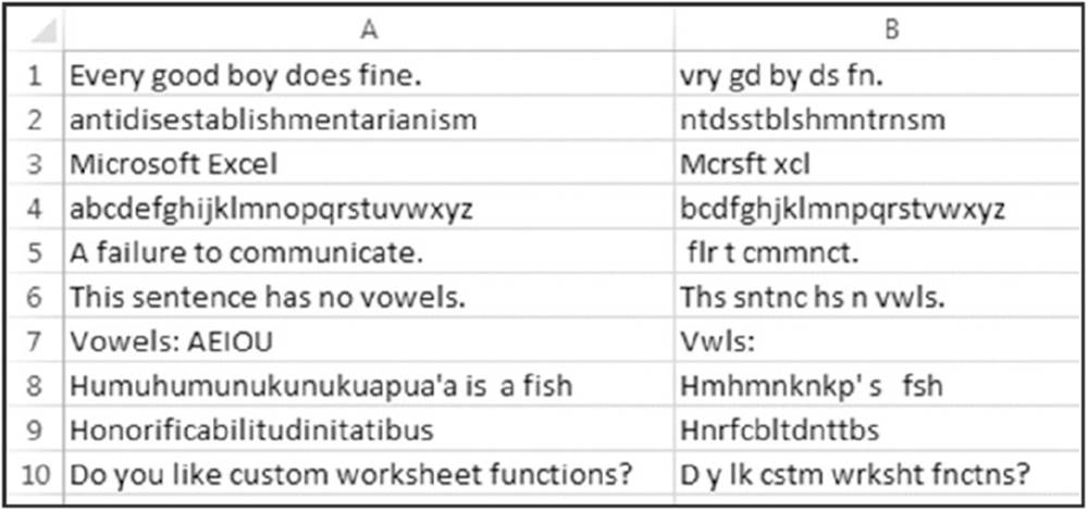
Figure 5.1 Using a custom function in a worksheet formula.

Actually, the function works like any built-in worksheet function. You can insert it in a formula by choosing Formulas ➜ Function Library ➜ Insert Function or by clicking the Insert Function Wizard icon to the left of the formula bar. Either of these actions displays the Insert Function dialog box. In the Insert Function dialog box, your custom functions are located, by default, in the User Defined category.

You can also nest custom functions and combine them with other elements in your formulas. For example, the following formula nests the REMOVEVOWELS function inside Excel’s UPPER function. The result is the original string (sans vowels), converted to uppercase.

=UPPER(REMOVEVOWELS(A1))

Using the function in a VBA procedure

In addition to using custom functions in worksheet formulas, you can use them in other VBA procedures. The following VBA procedure, which is defined in the same module as the custom REMOVEVOWELS function, first displays an input box to solicit text from the user. Then the procedure uses the VBA built-in MsgBox function to display the user input after the REMOVEVOWELS function processes it (see Figure 5.2). The original input appears as the caption in the message box.

Sub ZapTheVowels()

Dim UserInput as String

UserInput = InputBox("Enter some text:")

MsgBox REMOVEVOWELS(UserInput), vbInformation, UserInput

End Sub

Figure 5.2 shows text entered into an input box, and the result displayed in a message box .

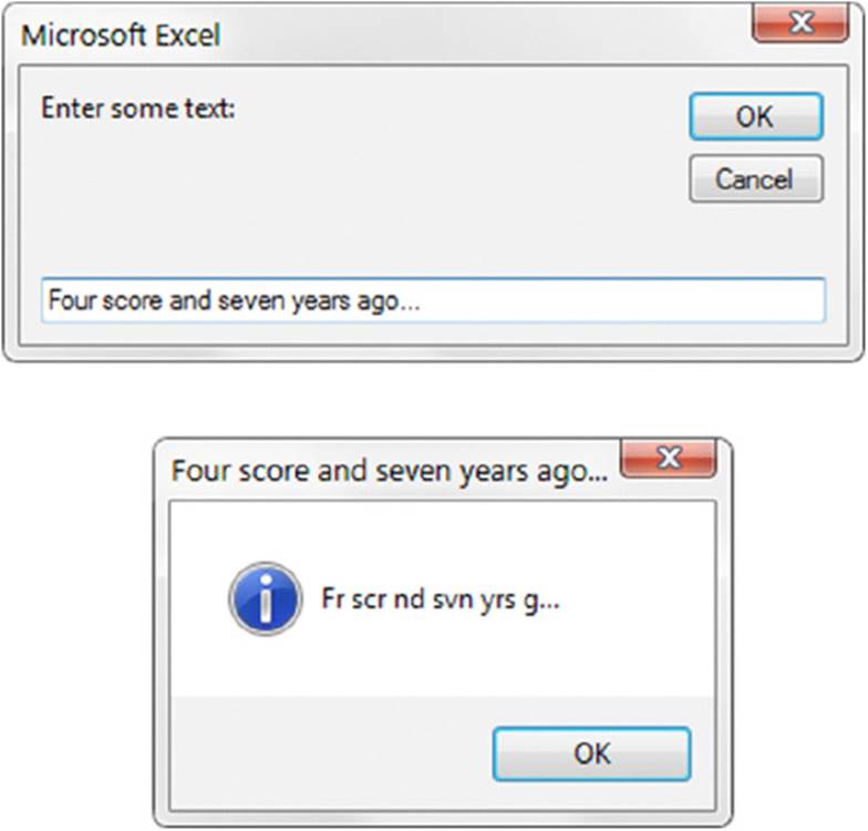
Figure 5.2 Using a custom function in a VBA procedure.

Analyzing the custom function

Function procedures can be as complex as you need them to be. Most of the time, they’re more complex and much more useful than this sample procedure. Nonetheless, an analysis of this example may help you understand what is happening.

Here’s the code, again:

Function REMOVEVOWELS(Txt) As String

' Removes all vowels from the Txt argument

Dim i As Long

REMOVEVOWELS =""

For i = 1 To Len(Txt)

If Not UCase(Mid(Txt, i, 1)) Like"[AEIOU]" Then

REMOVEVOWELS = REMOVEVOWELS & Mid(Txt, i, 1)

End If

Next i

End Function

Note that the procedure starts with the keyword Function, rather than Sub, followed by the name of the function (REMOVEVOWELS). This custom function uses only one argument (Txt), enclosed in parentheses. As String defines the data type of the function’s return value. Excel uses the Variant data type if no data type is specified.

The second line is an optional comment that describes what the function does. This line is followed by a Dim statement, which declares the variable (i) used in the procedure as type Long.

The next five instructions make up a For-Next loop. The procedure loops through each character in the input and builds the string. The first instruction in the loop uses VBA’s Mid function to return a single character from the input string and converts this character to uppercase. That character is then compared to a list of characters by using Excel’s Like operator. In other words, the If clause is true if the character isn’t A, E, I, O, or U. In such a case, the character is appended to the REMOVEVOWELS variable.

When the loop is finished, REMOVEVOWELS consists of the input string with all vowels removed. This string is the value that the function returns.

The procedure ends with an End Function statement.

Keep in mind that you can do the coding for this function in a number of different ways. Here’s a function that accomplishes the same result but is coded differently:

Function REMOVEVOWELS(txt) As String

' Removes all vowels from the Txt argument

Dim i As Long

Dim TempString As String

TempString =""

For i = 1 To Len(txt)

Select Case ucase(Mid(txt, i, 1))

Case"A","E","I","O","U"

'Do nothing

Case Else

TempString = TempString & Mid(txt, i, 1)

End Select

Next i

REMOVEVOWELS = TempString

End Function

In this version, we used a string variable (TempString) to store the vowel-less string as it’s being constructed. Then, before the procedure ends, we assigned the contents of TempString to the function’s name. This version also uses a Select Case construct rather than anIf-Then construct.

On the Web

Both versions of this function are available at this book’s website. The file is named remove vowels.xlsm.

What custom worksheet functions can’t do

When you develop custom functions, it’s important to understand a key distinction between functions that you call from other VBA procedures and functions that you use in worksheet formulas. Function procedures used in worksheet formulas must be passive. For example, code in a Function procedure can’t manipulate ranges or change things on the worksheet. An example can help make this limitation clear.

You may be tempted to write a custom worksheet function that changes a cell’s formatting. For example, it may be useful to have a formula that uses a custom function to change the color of text in a cell based on the cell’s value. Try as you might, however, such a function is impossible to write. No matter what you do, the function won’t change the worksheet. Remember, a function simply returns a value. It can’t perform actions with objects.

That said, we should point out one notable exception. You can change the text in a cell comment by using a custom VBA function. Here’s an example function that does just that:

Function MODIFYCOMMENT(Cell As Range, Cmt As String)

Cell.Comment.Text Cmt

End Function

Here’s an example of using this function in a formula. The formula replaces the comment in cell A1 with new text. The function won’t work if cell A1 doesn’t have a comment.

=MODIFYCOMMENT(A1,"Hey, I changed your comment")

Function Procedures

A Function procedure has much in common with a Sub procedure. (For more information on Sub procedures, see Chapter 4.)

The syntax for declaring a function is as follows:

[Public | Private][Static] Function name ([arglist])[As type]

[instructions]

[name = expression]

[Exit Function]

[instructions]

[name = expression]

End Function

The Function procedure contains the following elements:

· Public: Optional. Indicates that the Function procedure is accessible to all other procedures in all other modules in all active Excel VBA projects.

· Private: Optional. Indicates that the Function procedure is accessible only to other procedures in the same module.

· Static: Optional. Indicates that the values of variables declared in the Function procedure are preserved between calls.

· Function: Required. Indicates the beginning of a procedure that returns a value or other data.

· name: Required. Any valid Function procedure name, which must follow the same rules as a variable name.

· arglist: Optional. A list of one or more variables that represent arguments passed to the Function procedure. The arguments are enclosed in parentheses. Use a comma to separate pairs of arguments.

· type: Optional. The data type returned by the Function procedure.

· instructions: Optional. Any number of valid VBA instructions.

· Exit Function: Optional. A statement that forces an immediate exit from the Function procedure before its completion.

· End Function: Required. A keyword that indicates the end of the Function procedure.

A key point to remember about a custom function written in VBA is that a value is always assigned to the function’s name a minimum of one time, generally when it has completed execution.

To create a custom function, start by inserting a VBA module. You can use an existing module, as long as it’s a normal VBA module. Enter the keyword Function, followed by the function name and a list of its arguments (if any) in parentheses. You can also declare the data type of the return value by using the As keyword (this step is optional but recommended). Insert the VBA code that performs the work, making sure that the appropriate value is assigned to the term corresponding to the function name at least once in the body of the Function procedure. End the function with an End Function statement.

Function names must adhere to the same rules as variable names. If you plan to use your custom function in a worksheet formula, be careful if the function name is also a cell address. For example, if you use something such as ABC123 as a function name, you can’t use the function in a worksheet formula because ABC123 is a cell address. If you do so, Excel displays a #REF! error.

The best advice is to avoid using function names that are also cell references, including named ranges. And avoid using function names that correspond to Excel’s built-in function names. In the case of a function name conflict, Excel always uses its built-in function.

A function’s scope

In Chapter 4, we discuss the concept of a procedure’s scope (public or private). The same discussion applies to functions: A function’s scope determines whether it can be called by procedures in other modules or in worksheets.

Here are a few things to keep in mind about a function’s scope:

· If you don’t declare a function’s scope, its default scope is Public.

· Functions declared As Private don’t appear in Excel’s Insert Function dialog box. Therefore, when you create a function that should be used only in a VBA procedure, you should declare it Private so that users don’t try to use it in a formula.

· If your VBA code needs to call a function that’s defined in another workbook, set up a reference to the other workbook by choosing the Visual Basic Editor (VBE) Tools ➜ References command.

· You do not have to establish a reference if the function is defined in an add-in. Such a function is available for use in all workbooks.

Executing function procedures

Although you can execute a Sub procedure in many ways, you can execute a Function procedure in only four ways:

· Call it from another procedure

· Use it in a worksheet formula

· Use it in a formula that’s used to specify conditional formatting

· Call it from the VBE Immediate window

From a procedure

You can call custom functions from a VBA procedure the same way that you call built-in functions. For example, after you define a function called SUMARRAY, you can enter a statement like the following:

Total = SUMARRAY(MyArray)

This statement executes the SUMARRAY function with MyArray as its argument, returns the function’s result, and assigns it to the Total variable.

You also can use the Run method of the Application object. Here’s an example:

Total = Application.Run ("SUMARRAY","MyArray")

The first argument for the Run method is the function name. Subsequent arguments represent the arguments for the function. The arguments for the Run method can be literal strings (as shown in the preceding example), numbers, expressions, or variables.

In a worksheet formula

Using custom functions in a worksheet formula is like using built-in functions except that you must ensure that Excel can locate the Function procedure. If the Function procedure is in the same workbook, you don’t have to do anything special. If it’s in a different workbook, you may have to tell Excel where to find it.

You can do so in three ways:

· Precede the function name with a file reference. For example, if you want to use a function called COUNTNAMES that’s defined in an open workbook named Myfuncs.xlsm, you can use the following reference:

·=Myfuncs.xlsm!COUNTNAMES(A1:A1000)

If you insert the function with the Insert Function dialog box, the workbook reference is inserted automatically.

· Set up a reference to the workbook. You do so by choosing the VBE Tools ➜ References command. If the function is defined in a referenced workbook, you don’t need to use the worksheet name. Even when the dependent workbook is assigned as a reference, the Paste Function dialog box continues to insert the workbook reference (although it’s not necessary).

· Create an add-in. When you create an add-in from a workbook that has Function procedures, you don’t need to use the file reference when you use one of the functions in a formula. The add-in must be installed, however. We discuss add-ins in Chapter 16.

You’ll notice that unlike Sub procedures, your Function procedures don’t appear in the Macro dialog box when you issue the Developer ➜ Code ➜ Macros command. In addition, you can’t choose a function when you issue the VBE Run ➜ Sub/UserForm command (or press F5) if the cursor is located in a Function procedure. (You get the Macro dialog box that lets you choose a macro to run.) Therefore, you need to do a bit of extra up-front work to test your functions while you’re developing them. One approach is to set up a simple procedure that calls the function. If the function is designed to be used in worksheet formulas, you’ll want to enter a simple formula to test it.

In a conditional formatting formula

When you specify conditional formatting, one of the options is to create a formula. The formula must be a logical formula (that is, it must return either TRUE or FALSE). If the formula returns TRUE, the condition is met and formatting is applied to the cell.

You can use custom VBA functions in your conditional formatting formulas. For example, here’s a simple VBA function that returns TRUE if its argument is a cell that contains a formula:

Function CELLHASFORMULA(cell) As Boolean

CELLHASFORMULA = cell.HasFormula

End Function

After defining this function in a VBA module, you can set up a conditional formatting rule so that cells that contain a formula contain different formatting:

1. Select the range that will contain the conditional formatting.

For example, select A1:G20.

2. Choose Home ➜ Styles ➜ Conditional Formatting ➜ New Rule.

3. In the New Formatting Rule dialog box, select the option labeled Use a Formula to Determine Which Cells to Format.

4. Enter this formula in the formula box — but make sure that the cell reference argument corresponds to the upper-left cell in the range that you selected in Step 1:

=CELLHASFORMULA(A1)

5. Click the Format button to specify the formatting for cells that meet this condition.

6. Click OK to apply the conditional formatting rule to the selected range.

Cells in the range that contain a formula will display the formatting you specified. In the New Formatting Rule dialog box shown in Figure 5.3, we are specifying a custom function in a formula.

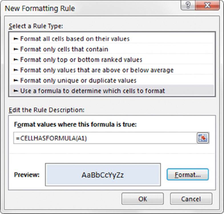
Figure 5.3 Using a custom VBA function for conditional formatting.

The ISFORMULA worksheet function (introduced in Excel 2013) works exactly like the custom CELLHASFORMULA function. But the CELLHASFORMULA function is still useful if you plan to share your workbook with others who are still using Excel 2010 or earlier versions.

From the VBE Immediate Window

The final way to call a Function procedure is from the VBE Immediate window. This method is generally used only for testing. Figure 5.4 shows an example. The ? character is a shortcut for print.

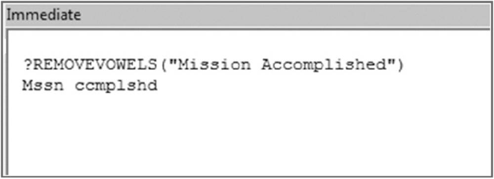
Figure 5.4 Calling a Function procedure from the Immediate window.

Function Arguments

Keep in mind the following points about Function procedure arguments:

· Arguments can be variables (including arrays), constants, literals, or expressions.

· Some functions don’t have arguments.

· Some functions have a fixed number of required arguments (from 1 to 60).

· Some functions have a combination of required and optional arguments.

Note

If your formula uses a custom worksheet function and it returns #VALUE!, your function has an error. The error may be caused by logical errors in your code or by passing incorrect arguments to the function. See the section “Debugging Functions,” later in this chapter.

Function Examples

In this section, we present a series of examples that demonstrate how to use arguments effectively with functions. By the way, this discussion applies also to Sub procedures.

Functions with no argument

Like Sub procedures, Function procedures need not have arguments. Excel, for example, has a few built-in functions that don’t use arguments, including RAND, TODAY, and NOW. You can create similar functions.

This section contains examples of functions that don’t use an argument.

On the Web

A workbook that contains these functions is available on this book’s website. The file is named no argument.xlsm.

Here’s a simple example of a function that doesn’t use an argument. The following function returns the UserName property of the Application object. This is the name that appears in the Excel Options dialog box (General tab) and is stored in the Windows Registry.

Function USER()

' Returns the name of the current user

USER = Application.UserName

End Function

When you enter the following formula, the cell returns the name of the current user:

=USER()

Note

When you use a function with no arguments in a worksheet formula, you must include a set of empty parentheses. This requirement isn’t necessary if you call the function in a VBA procedure, although including the empty parentheses does make it clear that you’re calling a function.

There is no need to use this function in another procedure because you can simply access the UserName property directly in your code.

The USER function demonstrates how you can create a wrapper function that returns a property or the result of a VBA function. Following are three additional wrapper functions that take no argument:

Function EXCELDIR() As String

' Returns the directory in which Excel is installed

EXCELDIR = Application.Path

End Function

Function SHEETCOUNT()

' Returns the number of sheets in the workbook

SHEETCOUNT = Application.Caller.Parent.Parent.Sheets.Count

End Function

Function SHEETNAME()

' Returns the name of the worksheet

SHEETNAME = Application.Caller.Parent.Name

End Function

You can probably think of other potentially useful wrapper functions. For example, you can write a function to display the template’s location (Application.TemplatesPath), the default file location (Application.DefaultFilePath), and the version of Excel (Application.Version). Also, note that Excel 2013 introduced a worksheet function, SHEETS, that makes the SHEETCOUNT function obsolete.

Here’s another example of a function that doesn’t take an argument. Most people use Excel’s RAND function to quickly fill a range of cells with values. But the RAND function forces random values to be changed whenever the worksheet was recalculated, So after using the RAND function, most people will, convert the formulas to values.

As an alternative, you could use VBA to create a custom function that returns static random numbers that do not change. The custom function follows:

Function STATICRAND()

' Returns a random number that doesn't

' change when recalculated

STATICRAND = Rnd()

End Function

If you want to generate a series of random integers between 0 and 1,000, you can use a formula such as this:

=INT(STATICRAND()*1000)

The values produced by this formula never change when the worksheet is calculated normally. However, you can force the formula to recalculate by pressing Ctrl+Alt+F9.

Controlling function recalculation

When you use a custom function in a worksheet formula, when is it recalculated?

Custom functions behave like Excel’s built-in worksheet functions. Normally, a custom function is recalculated only when it needs to be — which is only when any of the function’s arguments are modified. You can, however, force functions to recalculate more frequently. Adding the following statement to a Function procedure makes the function recalculate whenever the sheet is recalculated. If you’re using automatic calculation mode, a calculation occurs whenever any cell is changed.

Application.Volatile True

The Volatile method of the Application object has one argument (either True or False). Marking a Function procedure as volatile forces the function to be calculated whenever recalculation occurs for any cell in the worksheet.

For example, the custom STATICRAND function can be changed to emulate Excel’s RAND function using the Volatile method:

Function NONSTATICRAND()

' Returns a random number that changes with each calculation

Application.Volatile True

NONSTATICRAND = Rnd()

End Function

Using the False argument of the Volatile method causes the function to be recalculated only when one or more of its arguments change as a result of a recalculation.

To force an entire recalculation, including nonvolatile custom functions, press Ctrl+Alt+F9. This key combination will, for example, generate new random numbers for the STATICRAND function presented in this chapter.

A function with one argument

This section describes a function for sales managers who need to calculate the commissions earned by their sales forces. The calculations in this example are based on the following table:

Note that the commission rate is nonlinear and also depends on the month’s total sales. Employees who sell more earn a higher commission rate.

You can calculate commissions for various sales amounts entered in a worksheet in several ways. If you’re not thinking too clearly, you can waste lots of time and come up with a lengthy formula such as this one:

=IF(AND(A1>=0,A1<=9999.99),A1*0.08,

IF(AND(A1>=10000,A1<=19999.99),A1*0.105,

IF(AND(A1>=20000,A1<=39999.99),A1*0.12,

IF(A1>=40000,A1*0.14,0))))

This approach is bad for a couple of reasons. First, the formula is overly complex, making it difficult to understand. Second, the values are hard-coded into the formula, making the formula difficult to modify.

A better (non-VBA) approach is to use a lookup table function to compute the commissions. For example, the following formula uses VLOOKUP to retrieve the commission value from a range named Table and multiplies that value by the value in cell A1:

=VLOOKUP(A1,Table,2)*A1

Yet another approach (which eliminates the need to use a lookup table) is to create a custom function such as the following:

Function COMMISSION(Sales)

Const Tier1 = 0.08

Const Tier2 = 0.105

Const Tier3 = 0.12

Const Tier4 = 0.14

' Calculates sales commissions

Select Case Sales

Case 0 To 9999.99: COMMISSION = Sales * Tier1

Case 10000 To 19999.99: COMMISSION = Sales * Tier2

Case 20000 To 39999.99: COMMISSION = Sales * Tier3

Case Is >= 40000: COMMISSION = Sales * Tier4

End Select

End Function

After you enter this function in a VBA module, you can use it in a worksheet formula or call the function from other VBA procedures.

Entering the following formula into a cell produces a result of 3,000; the amount (25,000) qualifies for a commission rate of 12 percent:

=COMMISSION(25000)

Even if you don’t need custom functions in a worksheet, creating Function procedures can make your VBA coding much simpler. For example, if your VBA procedure calculates sales commissions, you can use the same function and call it from a VBA procedure. Here’s a tiny procedure that asks the user for a sales amount and then uses the COMMISSION function to calculate the commission due:

Sub CalcComm()

Dim Sales as Long

Sales = InputBox("Enter Sales:")

MsgBox"The commission is" & COMMISSION(Sales)

End Sub

The CalcComm procedure starts by displaying an input box that asks for the sales amount. Then it displays a message box with the calculated sales commission for that amount.

This Sub procedure works, but it’s crude. Following is an enhanced version with a bit of error handling. It also displays formatted values and keeps looping until the user clicks No (see Figure 5.5).

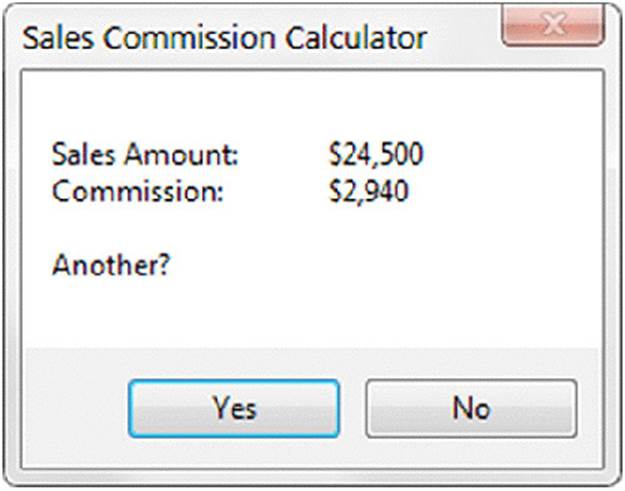
Figure 5.5 Using a function to display the result of a calculation.

Sub CalcComm()

Dim Sales As Long

Dim Msg As String, Ans As String

' Prompt for sales amount

Sales = Val(InputBox("Enter Sales:", _

"Sales Commission Calculator"))

' Exit if canceled

If Sales = 0 Then Exit Sub

' Build the Message

Msg ="Sales Amount:" & vbTab & Format(Sales,"$#,##0.00")

Msg = Msg & vbCrLf &"Commission:" & vbTab

Msg = Msg & Format(COMMISSION(Sales),"$#,##0.00")

Msg = Msg & vbCrLf & vbCrLf &"Another?"

' Display the result and prompt for another

Ans = MsgBox(Msg, vbYesNo,"Sales Commission Calculator")

If Ans = vbYes Then CalcComm

End Sub

This function uses two VBA built-in constants: vbTab represents a tab (to space the output), and vbCrLf specifies a carriage return and line feed (to skip to the next line). VBA’s Format function displays a value in a specified format (in this case, with a dollar sign, a comma, and two decimal places).

In both examples, the Commission function must be available in the active workbook; otherwise, Excel displays an error message saying that the function isn’t defined.

Use arguments, not cell references

All ranges that are used in a custom function should be passed as arguments. Consider the following function, which returns the value in A1, multiplied by 2:

Function DOUBLECELL()

DOUBLECELL = Range("A1") * 2

End Function

Although this function works, at times it may return an incorrect result. Excel’s calculation engine can’t account for ranges in your code that aren’t passed as arguments. Therefore, in some cases, all precedents may not be calculated before the function’s value is returned. The DOUBLECELL function should be written as follows, with A1 passed as the argument:

Function DOUBLECELL(cell)

DOUBLECELL = cell * 2

End Function

A function with two arguments

Imagine that the aforementioned hypothetical sales managers implement a new policy to help reduce turnover: The total commission paid is increased by 1 percent for every year that the salesperson has been with the company.

We modified the custom COMMISSION function (defined in the preceding section) so that it takes two arguments. The new argument represents the number of years. Call this new function COMMISSION2:

Function COMMISSION2(Sales, Years)

' Calculates sales commissions based on

' years in service

Const Tier1 = 0.08

Const Tier2 = 0.105

Const Tier3 = 0.12

Const Tier4 = 0.14

Select Case Sales

Case 0 To 9999.99: COMMISSION2 = Sales * Tier1

Case 10000 To 19999.99: COMMISSION2 = Sales * Tier2

Case 20000 To 39999.99: COMMISSION2 = Sales * Tier3

Case Is >= 40000: COMMISSION2 = Sales * Tier4

End Select

COMMISSION2 = COMMISSION2 + (COMMISSION2 * Years / 100)

End Function

Pretty simple, right? We just added the second argument (Years) to the Function statement and included an additional computation that adjusts the commission.

Here’s an example of how you can write a formula using this function (it assumes that the sales amount is in cell A1 and the number of years the salesperson has worked is in cell B1):

=COMMISSION2(A1,B1)

On the Web

All commission-related examples are available on this book’s website, in a file named commission functions.xlsm.

A function with an array argument

A Function procedure also can accept one or more arrays as arguments, process the array(s), and return a single value. The array can also consist of a range of cells.

The following function accepts an array as its argument and returns the sum of its elements:

Function SUMARRAY(List) As Double

Dim Item As Variant

SumArray = 0

For Each Item In List

If WorksheetFunction.IsNumber(Item) Then _

SUMARRAY = SUMARRAY + Item

Next Item

End Function

Excel’s ISNUMBER function checks to see whether each element is a number before adding it to the total. Adding this simple error-checking statement eliminates the type-mismatch error that occurs when you try to perform arithmetic with something other than a number.

The following procedure demonstrates how to call this function from a Sub procedure. The MakeList procedure creates a 100-element array and assigns a random number to each element. Then the MsgBox function displays the sum of the values in the array by calling the SUMARRAY function.

Sub MakeList()

Dim Nums(1 To 100) As Double

Dim i As Integer

For i = 1 To 100

Nums(i) = Rnd * 1000

Next i

MsgBox SUMARRAY(Nums)

End Sub

Note that the SUMARRAY function doesn’t declare the data type of its argument (it’s a variant). Because it’s not declared as a specific numeric type, the function also works in your worksheet formulas in which the argument is a Range object. For example, the following formula returns the sum of the values in A1:C10:

=SUMARRAY(A1:C10)

You might notice that, when used in a worksheet formula, the SUMARRAY function works very much like Excel’s SUM function. One difference, however, is that SUMARRAY doesn’t accept multiple arguments. Understand that this example is for educational purposes only. Using the SUMARRAY function in a formula offers no advantages over the Excel SUM function.

On the Web

This example, named array argument.xlsm, is available on this book’s website.

A function with optional arguments

Many of Excel’s built-in worksheet functions use optional arguments. An example is the LEFT function, which returns characters from the left side of a string. Its syntax is:

LEFT(text,num_chars)

The first argument is required, but the second is optional. If the optional argument is omitted for the LEFT function, Excel assumes a value of 1. Therefore, the following two formulas return the same result:

=LEFT(A1,1)

=LEFT(A1)

The custom functions that you develop in VBA also can have optional arguments. You specify an optional argument by preceding the argument’s name with the keyword Optional. In the argument list, optional arguments must appear after any required arguments.

Following is a simple function example that returns the user’s name. The function’s argument is optional.

Function USER(Optional UpperCase As Variant)

If IsMissing(UpperCase) Then UpperCase = False

USER = Application.UserName

If UpperCase Then USER = UCase(USER)

End Function

If the argument is False or omitted, the user’s name is returned without any changes. If the argument is True, the user’s name is converted to uppercase (using the VBA UCase function) before it’s returned. Note that the first statement in the procedure uses the VBAIsMissing function to determine whether the argument was supplied. If the argument is missing, the statement sets the UpperCase variable to False (the default value).

All the following formulas are valid, and the first two produce the same result:

=USER()

=USER(False)

=USER(True)

Note

If you need to determine whether an optional argument was passed to a function, you must declare the optional argument as a Variant data type. Then you can use the IsMissing function in the procedure, as demonstrated in this example. In other words, the argument for the IsMissing function must always be a Variant data type.

The following is another example of a custom function that uses an optional argument. This function randomly chooses one cell from an input range and returns that cell’s contents. If the second argument is True, the selected value changes whenever the worksheet is recalculated (that is, the function is made volatile). If the second argument is False (or omitted), the function isn’t recalculated unless one of the cells in the input range is modified.

Function DRAWONE(Rng As Variant, Optional Recalc As Variant = False)

' Chooses one cell at random from a range

' Make function volatile if Recalc is True

Application.Volatile Recalc

' Determine a random cell

DRAWONE = Rng(Int((Rng.Count) * Rnd + 1))

End Function

Note that the second argument for DRAWONE includes the Optional keyword, along with a default value.

All the following formulas are valid, and the first two have the same effect:

=DRAWONE(A1:A100)

=DRAWONE(A1:A100,False)

=DRAWONE(A1:A100,True)

This function might be useful for choosing lottery numbers, picking a winner from a list of names, and so on.

On the Web

This function is available on this book’s website. The filename is draw.xlsm.

A function that returns a VBA array

VBA includes a useful function called Array. The Array function returns a variant that contains an array (that is, multiple values). If you’re familiar with array formulas in Excel, you have a head start on understanding VBA’s Array function. You enter an array formula into a cell by pressing Ctrl+Shift+Enter. Excel inserts curly braces around the formula to indicate that it’s an array formula.

Note

It’s important to understand that the array returned by the Array function isn’t the same as a normal array made up of elements of the Variant data type. In other words, a variant array isn’t the same as an array of variants.

The MONTHNAMES function, which follows, is a simple example that uses VBA’s Array function in a custom function:

Function MONTHNAMES ()

MONTHNAMES = Array("Jan","Feb","Mar","Apr","May","Jun", _

"Jul","Aug","Sep","Oct","Nov","Dec")

End Function

The MONTHNAMES function returns a horizontal array of month names. You can create a multicell array formula that uses the MONTHNAMES function. Here’s how to use it: Make sure that the function code is present in a VBA module. Next, in a worksheet, select multiple cells in a row (start by selecting 12 cells). Then enter the formula that follows (without the braces) and press Ctrl+Shift+Enter:

{=MONTHNAMES()}

What if you’d like to generate a vertical list of month names? No problem; just select a vertical range, enter the following formula (without the braces), and then press Ctrl+Shift+Enter:

{=TRANSPOSE(MONTHNAMES ())}

This formula uses the Excel TRANSPOSE function to convert the horizontal array to a vertical array.

The following example is a variation on the MONTHNAMES function:

Function MonthNames(Optional MIndex)

Dim AllNames As Variant

Dim MonthVal As Long

AllNames = Array("Jan","Feb","Mar","Apr","May","Jun", _

"Jul","Aug","Sep","Oct","Nov","Dec")

If IsMissing(MIndex) Then

MONTHNAMES = AllNames

Else

Select Case MIndex

Case Is >= 1

' Determine month value (for example, 13=1)

MonthVal = ((MIndex - 1) Mod 12)

MONTHNAMES = AllNames(MonthVal)

Case Is <= 0 ' Vertical array

MONTHNAMES = Application.Transpose(AllNames)

End Select

End If

End Function

Note that we use the VBA IsMissing function to test for a missing argument. In this situation, it isn’t possible to specify the default value for the missing argument in the argument list of the function because the default value is defined in the function. You can use theIsMissing function only if the optional argument is a variant.

This enhanced function uses an optional argument that works as follows:

· If the argument is missing, the function returns a horizontal array of month names.

· If the argument is less than or equal to 0, the function returns a vertical array of month names. It uses Excel’s TRANSPOSE function to convert the array.

· If the argument is greater than or equal to 1, the function returns the month name that corresponds to the argument value.

Note

This procedure uses the Mod operator to determine the month value. The Mod operator returns the remainder after dividing the first operand by the second. Keep in mind that the AllNames array is zero-based and that indices range from 0 to 11. In the statement that uses the Mod operator, 1 is subtracted from the function’s argument. Therefore, an argument of 13 returns 0 (corresponding to Jan), and an argument of 24 returns 11 (corresponding to Dec).

You can use this function in a number of ways, as illustrated in Figure 5.6.

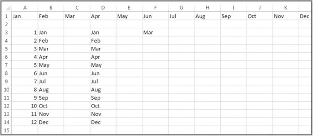
Figure 5.6 Different ways of passing an array or a single value to a worksheet.

Range A1:L1 contains the following formula entered as an array. Start by selecting A1:L1, enter the formula (without the braces), and then press Ctrl+Shift+Enter.

{=MONTHNAMES()}

Range A3:A14 contains integers from 1 to 12. Cell B3 contains the following (nonarray) formula, which was copied to the 11 cells below it:

=MONTHNAMES(A3)

Range D3:D14 contains the following formula entered as an array:

{=MONTHNAMES(-1)}

Cell F3 contains this (nonarray) formula:

=MONTHNAMES(3)

To enter an array formula, you must press Ctrl+Shift+Enter (and don’t enter the curly braces).

Note

The lower bound of an array, created using the Array function, is determined by the lower bound specified with the Option Base statement at the top of the module. If there is no Option Base statement, the default lower bound is 0.

A workbook that demonstrates the MONTHNAMES function is available on this book’s website. The file is named month names.xslm.

A function that returns an error value

In some cases, you might want your custom function to return a particular error value. Consider the REMOVEVOWELS function, which we presented earlier in this chapter:

Function REMOVEVOWELS(Txt) As String

' Removes all vowels from the Txt argument

Dim i As Long

RemoveVowels =""

For i = 1 To Len(Txt)

If Not UCase(Mid(Txt, i, 1)) Like"[AEIOU]" Then

REMOVEVOWELS = REMOVEVOWELS & Mid(Txt, i, 1)

End If

Next i

End Function

When used in a worksheet formula, this function removes the vowels from its single-cell argument. If the argument is a numeric value, this function returns the value as a string. You may prefer that the function returns an error value (#N/A), rather than the numeric value converted to a string.

You may be tempted simply to assign a string that looks like an Excel formula error value. For example:

REMOVEVOWELS ="#N/A"

Although the string looks like an error value, other formulas that may reference it don’t treat it as such. To return a real error value from a function, use the VBA CVErr function, which converts an error number to a real error.

Fortunately, VBA has built-in constants for the errors that you want to return from a custom function. These errors are Excel formula error values and not VBA runtime error values. These constants are as follows:

· xlErrDiv0 (for #DIV/0!)

· xlErrNA (for #N/A)

· xlErrName (for #NAME?)

· xlErrNull (for #NULL!)

· xlErrNum (for #NUM!)

· xlErrRef (for #REF!)

· xlErrValue (for #VALUE!)

To return a #N/A error from a custom function, you can use a statement like this:

REMOVEVOWELS = CVErr(xlErrNA)

The revised REMOVEVOWELS function follows. This function uses an If-Then construct to take a different action if the argument isn’t text. It uses Excel’s ISTEXT function to determine whether the argument is text. If the argument is text, the function proceeds normally. If the cell doesn’t contain text (or is empty), the function returns the #N/A error.

Function REMOVEVOWELS (Txt) As Variant

' Removes all vowels from the Txt argument

' Returns #VALUE if Txt is not a string

Dim i As Long

RemoveVowels =""

If Application.WorksheetFunction.IsText(Txt) Then

For i = 1 To Len(Txt)

If Not UCase(Mid(Txt, i, 1)) Like"[AEIOU]" Then

REMOVEVOWELS = REMOVEVOWELS & Mid(Txt, i, 1)

End If

Next i

Else

REMOVEVOWELS = CVErr(xlErrNA)

End If

End Function

Note

Note that we also changed the data type for the function’s return value. Because the function can now return something other than a string, we changed the data type to Variant.

A function with an indefinite number of arguments

Some Excel worksheet functions take an indefinite number of arguments. A familiar example is the SUM function, which has the following syntax:

SUM(number1,number2,...)

The first argument is required, but you can specify as many as 254 additional arguments. Here’s an example of a SUM function with four range arguments:

=SUM(A1:A5,C1:C5,E1:E5,G1:G5)

You can even mix and match the argument types. For example, the following example uses three arguments: The first is a range, the second is a value, and the third is an expression.

=SUM(A1:A5,12,24*3)

You can create Function procedures that have an indefinite number of arguments. The trick is to use an array as the last (or only) argument, preceded by the keyword ParamArray.

Note

ParamArray can apply only to the last argument in the procedure’s argument list. It’s always a Variant data type and always an optional argument (although you don’t use the Optional keyword).

Following is a function that can have any number of single-value arguments. (It doesn’t work with multicell range arguments.) It simply returns the sum of the arguments.

Function SIMPLESUM(ParamArray arglist() As Variant) As Double

For Each arg In arglist

SIMPLESUM = SIMPLESUM + arg

Next arg

End Function

To modify this function so that it works with multicell range arguments, you need to add another loop, which processes each cell in each of the arguments:

Function SIMPLESUM (ParamArray arglist() As Variant) As Double

Dim cell As Range

For Each arg In arglist

For Each cell In arg

SIMPLESUM = SIMPLESUM + cell

Next cell

Next arg

End Function

The SIMPLESUM function is similar to Excel’s SUM function, but it’s not nearly as flexible. Try it by using various types of arguments, and you’ll see that it fails if any of the cells contain a nonvalue, or even if you use a literal value for an argument.

Emulating Excel’s SUM Function

In this section, we present a custom function called MYSUM. Unlike the SIMPLESUM function listed in the preceding section, the MYSUM function emulates Excel’s SUM function (almost) perfectly.

Before you look at the code for MYSUM, take a minute to think about the Excel SUM function. It is versatile: It can have as many as 255 arguments (even “missing” arguments), and the arguments can be numerical values, cells, ranges, text representations of numbers, logical values, and even embedded functions. For example, consider the following formula:

=SUM(B1,5,"6",,TRUE,SQRT(4),A1:A5,D:D,C2*C3)

This perfectly valid formula contains all the following types of arguments, listed here in the order of their presentation:

· A single-cell reference

· A literal value

· A string that looks like a value

· A missing argument

· A logical TRUE value

· An expression that uses another function

· A simple range reference

· A range reference that includes an entire column

· An expression that calculates the product of two cells

The MYSUM function (see Listing 5-1) handles all these argument types.

On the Web

A workbook containing the MYSUM function is available on this book’s website. The file is named mysum function.xlsm.

Listing 5-1: MYSUM Function

Function MYSUM(ParamArray args() As Variant) As Variant

' Emulates Excel's SUM function

' Variable declarations

Dim i As Variant

Dim TempRange As Range, cell As Range

Dim ECode As String

Dim m, n

MYSUM = 0

' Process each argument

For i = 0 To UBound(args)

' Skip missing arguments

If Not IsMissing(args(i)) Then

' What type of argument is it?

Select Case TypeName(args(i))

Case"Range"

' Create temp range to handle full row or column ranges

Set TempRange = Intersect(args(i).Parent.UsedRange, args(i))

For Each cell In TempRange

If IsError(cell) Then

MYSUM = cell ' return the error

Exit Function

End If

If cell = True Or cell = False Then

MYSUM = MYSUM + 0

Else

If IsNumeric(cell) Or IsDate(cell) Then _

MYSUM = MYSUM + cell

End If

Next cell

Case"Variant()"

n = args(i)

For m = LBound(n) To UBound(n)

MYSUM = MYSUM(MYSUM, n(m)) 'recursive call

Next m

Case"Null" 'ignore it

Case"Error" 'return the error

MYSUM = args(i)

Exit Function

Case"Boolean"

' Check for literal TRUE and compensate

If args(i) ="True" Then MYSUM = MYSUM + 1

Case"Date"

MYSUM = MYSUM + args(i)

Case Else

MYSUM = MYSUM + args(i)

End Select

End If

Next i

End Function

Figure 5.7 shows a workbook with various formulas that use SUM (column E) and MYSUM (column G). As you can see, the functions return identical results.

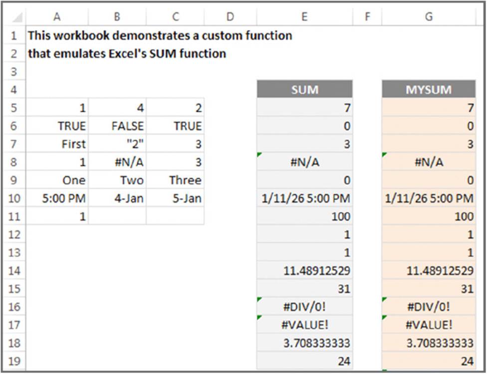
Figure 5.7 Comparing SUM with MYSUM.

MYSUM is a close emulation of the SUM function, but it’s not perfect. It cannot handle operations on arrays. For example, this array formula returns the sum of the squared values in range A1:A4:

{=SUM(A:A4^2)}

This formula returns a #VALUE! error:

{=MYSUM(A1:A4^2)}

If you’re interested in learning how the MYSUM function works, create a formula that uses the function. Then set a breakpoint in the code and step through the statements line by line. (See the section"Debugging Functions," later in this chapter.) Try this for several different argument types, and you’ll soon have a good feel for how the MYSUM function works.

As you study the code for MYSUM, keep the following points in mind:

· Missing arguments (determined by the IsMissing function) are simply ignored.

· The procedure uses the VBA TypeName function to determine the type of argument (Range, Error, and so on). Each argument type is handled differently.

· For a range argument, the function loops through each cell in the range, determines the type of data in the cell, and (if appropriate) adds its value to a running total.

· The data type for the function is Variant because the function needs to return an error if any of its arguments are an error value.

· If an argument contains an error (for example, #DIV/0!), the MYSUM function simply returns the error — just as Excel’s SUM function does.

· Excel’s SUM function considers a text string to have a value of 0 unless it appears as a literal argument (that is, as an actual value, not a variable). Therefore, MYSUM adds the cell’s value only if it can be evaluated as a number. (The VBA IsNumeric function is used to determine whether a string can be evaluated as a number.)

· For range arguments, the function uses the Intersect method to create a temporary range that consists of the intersection of the range and the sheet’s used range. This technique handles cases in which a range argument consists of a complete row or column, which would take forever to evaluate.

You may be curious about the relative speeds of SUM and MYSUM. The MYSUM function, of course, is much slower, but just how much slower depends on the speed of your system and the formulas themselves. However, the point of this example is not to create a new SUM function. Rather, it demonstrates how to create custom worksheet functions that look and work like those built into Excel.

Extended Date Functions

A common complaint among Excel users is the inability to work with dates prior to 1900. For example, genealogists often use Excel to keep track of birth and death dates. If either of those dates occurs in a year prior to 1900, calculating the number of years the person lived isn’t possible.

We created a series of functions that take advantage of the fact that VBA can work with a much larger range of dates. The earliest date recognized by VBA is January 1, 0100.

Caution

Beware of calendar changes if you use dates prior to 1752. Differences between the historical American, British, Gregorian, and Julian calendars can result in inaccurate computations.

The functions are:

· XDATE(y,m,d,fmt): Returns a date for a given year, month, and day. As an option, you can provide a date-formatting string.

· XDATEADD(xdate1,days,fmt): Adds a specified number of days to a date. As an option, you can provide a date-formatting string.

· XDATEDIF(xdate1,xdate2): Returns the number of days between two dates.

· XDATEYEARDIF(xdate1,xdate2): Returns the number of full years between two dates (useful for calculating ages).

· XDATEYEAR(xdate1): Returns the year of a date.

· XDATEMONTH(xdate1): Returns the month of a date.

· XDATEDAY(xdate1): Returns the day of a date.

· XDATEDOW(xdate1): Returns the day of the week of a date (as an integer between 1 and 7).

Figure 5.8 shows a workbook that uses some of these functions.

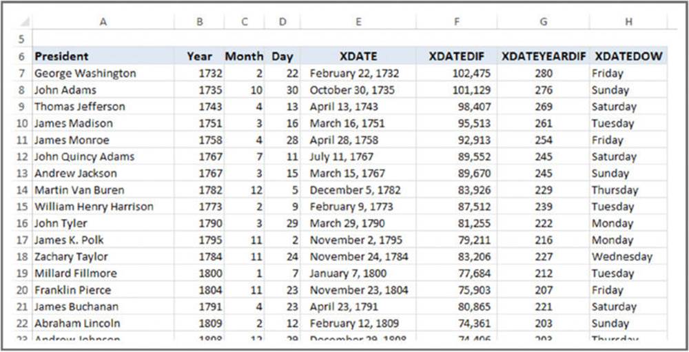
Figure 5.8 The Extended Date functions used in formulas.

Keep in mind that the date returned by these functions is a string, not a real date. Therefore, you can’t perform mathematical operations on the returned value using Excel’s standard operators. You can, however, use the return value as an argument for other Extended Date functions.

The functions are surprisingly simple. For example, here’s the listing for the XDATE function:

Function XDATE(y, m, d, Optional fmt As String) As String

If IsMissing(fmt) Then fmt ="Short Date"

XDATE = Format(DateSerial(y, m, d), fmt)

End Function

The arguments for XDATE are:

· y: Required. A four-digit year (0100–9999).

· m: Required. A month number (1–12).

· d: Required. A day number (1–31).

· fmt: Optional. A date format string.

If the fmt argument is omitted, the date is displayed using the system’s short date setting (as specified in the Windows Control Panel).

If the m or d argument exceeds a valid number, the date rolls over into the next year or month. For example, a month of 13 is interpreted as January of the next year.

On the Web

The VBA code for the Extended Data functions is available on this book’s website. The filename is extended date function.xlsm. You can also download documentation for these functions in the extended date functions help.pdf document.

Debugging Functions

When you’re using a formula in a worksheet to test a Function procedure, VBA runtime errors don’t appear in the all-too-familiar, pop-up error box. If an error occurs, the formula simply returns an error value (#VALUE!). The lack of a pop-up error message doesn’t present a problem for debugging functions because you have several possible workarounds:

· Place MsgBox functions at strategic locations to monitor the value of specific variables. Message boxes in Function procedures do pop up when the procedure is executed. But make sure that you have only one formula in the worksheet that uses your function; otherwise, message boxes will appear for each formula that is evaluated, which will quickly become annoying.

· Test the procedure by calling it from a Sub procedure, not from a worksheet formula. Runtime errors are displayed in the usual manner, and you can either fix the problem (if you know it) or jump right into using Debugger.

· Set a breakpoint in the function, and then step through the function. You then can access all standard VBA debugging tools. To set a breakpoint, move the cursor to the statement at which you want to pause execution and then choose Debug ➜ Toggle Breakpoint (or press F9). When the function is executing, press F8 to step through the procedure line-by-line.

· Use one or more temporary Debug.Print statements in your code to write values to the VBE Immediate window. For example, if you want to monitor a value inside a loop, use something like the following routine:

·Function VOWELCOUNT(r) As Long

· Dim Count As Long

· Dim i As Long

· Dim Ch As String * 1

· Count = 0

· For i = 1 To Len(r)

· Ch = UCase(Mid(r, i, 1))

· If Ch Like"[AEIOU]" Then

· Count = Count + 1

· Debug.Print Ch, i

· End If

· Next i

· VOWELCOUNT = Count

·End Function

In this case, the values of two variables, Ch and i, are printed to the Immediate window whenever the Debug.Print statement is encountered. Figure 5.9 shows the result when the function has an argument of Tucson, Arizona.

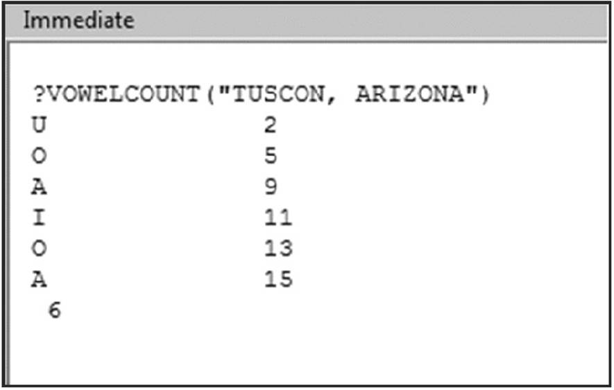
Figure 5.9 Use the Immediate window to display results while a function is running.

Dealing with the Insert Function Dialog Box

Excel’s Insert Function dialog box is a handy tool. When you’re creating a worksheet formula, this tool lets you select a particular worksheet function from a list of functions. These functions are grouped into various categories to make locating a particular function easier. When you select a function and click OK, the Function Arguments dialog box appears to help insert the function’s arguments.

The Insert Function dialog box also displays your custom worksheet functions. By default, custom functions are listed under the User Defined category. The Function Arguments dialog box prompts you for a custom function’s arguments.

The Insert Function dialog box enables you to search for a function by keyword. Unfortunately, you can’t use this search feature to locate custom functions created in VBA.

Note

Custom Function procedures defined with the Private keyword don’t appear in the Insert Function dialog box. If you develop a function that’s intended to be used only in your other VBA procedures, you should declare it by using the Private keyword. However, declaring the function as Private doesn’t prevent it from being used in a worksheet formula. It just prevents the display of the function in the Insert Function dialog box.

Using the MacroOptions method

You can use the MacroOptions method of the Application object to make your functions appear just like built-in functions. Specifically, this method enables you to:

· Provide a description of the function

· Specify a function category

· Provide descriptions for the function arguments

Another useful advantage of using the MacroOptions method is that it allows Excel to autocorrect the capitalization of your functions. For instance, if you create a function called MyFunction, and you enter the formula =myfunction(a), Excel will automatically change the formula to =MyFunction(a). This behavior provides a quick and easy way to tell if you’ve misspelled the function name (if the lower case letters do not autoadjust, the function name is misspelled).

Following is an example of a procedure that uses the MacroOptions method to provide information about a function:

Sub DescribeFunction()

Dim FuncName As String

Dim FuncDesc As String

Dim FuncCat As Long

Dim Arg1Desc As String, Arg2Desc As String

FuncName ="DRAWONE"

FuncDesc ="Displays the contents of a random cell from a range"

FuncCat = 5

Arg1Desc ="The range that contains the values"

Arg2Desc ="(Optional) If False or missing, a new cell is selected when"

Arg2Desc = Arg2Desc &"recalculated. If True, a new cell is selected"

Arg2Desc = Arg2Desc &"when recalculated."

Application.MacroOptions _

Macro:=FuncName, _

Description:=FuncDesc, _

Category:=FuncCat, _

ArgumentDescriptions:=Array(Arg1Desc, Arg2Desc)

End Sub

This procedure uses variables to store the information, and the variables are used as arguments for the MacroOptions method. The function is assigned to function category 5 (Lookup & Reference). Note that descriptions for the two arguments are indicated by using an array as the last argument for the MacroOptions method.

Note

The capability to provide argument descriptions was introduced in Excel 2010. If the workbook that contains the function is opened in a version prior to Excel 2010, the arguments won’t display the descriptions.

Figure 5.10 shows the Insert Function and Function Arguments dialog boxes after executing this procedure.

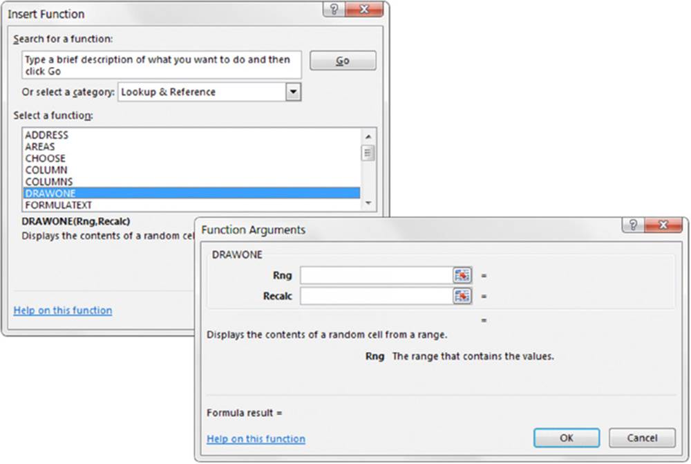
Figure 5.10 The Insert Function and Function Arguments dialog boxes for a custom function.

You need to execute the DescribeFunction procedure only one time. After doing so, the information assigned to the function is stored in the workbook. You can also omit arguments for the MacroOptions method. For example, if you don’t need the arguments to have descriptions, just omit the ArgumentDescriptions argument in the code.

Cross-Ref

For information on creating a custom help topic accessible from the Insert Function dialog box, refer to Chapter 19.

Specifying a function category

If you don’t use the MacroOptions method to specify a different category, your custom worksheet functions appear in the User Defined category in the Insert Function dialog box. You may prefer to assign your function to a different category. Assigning a function to a category also causes it to appear in the drop-down controls in the Formulas ➜ Function Library group on the Ribbon.

Table 5.1 lists the category numbers that you can use for the Category argument for the MacroOptions method. A few of these categories (10 through 13) aren’t normally displayed in the Insert Function dialog box. If you assign your function to one of these categories, the category will appear in the dialog box.

Table 5.1 Function Categories

*The Compatibility category was introduced in Excel 2010.

** The Web category was introduced in Excel 2013.

You can also create custom function categories. Instead of using a number for the Category argument for MacroOptions, use a text string. The statement that follows creates a new function category named VBA Functions and assigns the COMMISSIONfunction to this category:

Application.MacroOptions Macro:="COMMISSION",_

Category:="VBA Functions"

Adding a function description manually

As an alternative to using the MacroOptions method to provide a function description, you can use the Macro dialog box.

Note

If you don’t provide a description for your custom function, the Insert Function dialog box displays No help available.

Follow these steps to provide a description for a custom function:

1. Create your function in VBE.

2. Activate Excel, making sure that the workbook that contains the function is the active workbook.

3. Choose Developer ➜ Code ➜ Macros (or press Alt+F8).

The Macro dialog box lists available procedures, but your function won’t be in the list.

4. In the Macro Name box, type the name of your function.

5. Click the Options button to display the Macro Options dialog box.

6. In the Description box, enter the function description. The Shortcut Key field is irrelevant for functions.

7. Click OK and then click Cancel.

After you perform the preceding steps, the Insert Function dialog box displays the description that you entered in Step 6 when the function is selected.

Using Add-Ins to Store Custom Functions

You may prefer to store frequently used custom functions in an add-in file. A primary advantage is that you can use those functions in any workbook when the add-in is installed.

In addition, you can use the functions in formulas without a filename qualifier. Assume that you have a custom function named ZAPSPACES that is stored in Myfuncs.xlsm. To use this function in a formula in a workbook other than Myfuncs.xlsm, you need to enter the following formula:

=Myfuncs.xlsm!ZAPSPACES(A1)

If you create an add-in from Myfuncs.xlsm and the add-in is loaded, you can omit the file reference and enter a formula such as the following:

=ZAPSPACES(A1)

Note

We discuss add-ins in Chapter 16.

Caution

A potential problem with using add-ins to store custom functions is that your workbook is dependent on the add-in file. If you need to share your workbook with a colleague, you also need to share a copy of the add-in that contains the functions.

Using the Windows API

VBA can borrow methods from other files that have nothing to do with Excel or VBA — for example, the Dynamic Link Library (DLL) files that Windows and other software use. As a result, you can do things with VBA that would otherwise be outside the language’s scope.

The Windows Application Programming Interface (API) is a set of functions available to Windows programmers. When you call a Windows function from VBA, you’re accessing the Windows API. Many of the Windows resources used by Windows programmers are available in DLLs, which store programs and functions and are linked at runtime rather than at compile time.

64-bit Excel and API functions

Beginning with Excel 2010, using Windows API functions in your code became a bit more challenging because Excel became available in both 32-bit and 64-bit versions. If you want your code to be compatible with the 32-bit and the 64-bit versions of Excel, you need to declare your API functions twice, using compiler directives to ensure that the correct declaration is used.

For example, the following declaration works with 32-bit Excel versions but causes a compile error with 64-bit Excel:

Declare Function GetWindowsDirectoryA Lib"kernel32" _

(ByVal lpBuffer As String, ByVal nSize As Long) As Long

In many cases, making the declaration compatible with 64-bit Excel is as simple as adding PtrSafe after the Declare keyword. The following declaration is compatible with both the 32-bit and 64-bit versions of Excel:

Declare PtrSafe Function GetWindowsDirectoryA Lib"kernel32" _

(ByVal lpBuffer As String, ByVal nSize As Long) As Long

However, the code will fail in Excel 2007 and earlier versions because the PtrSafe keyword is not recognized by those versions.

In Chapter 21, we describe how to make API function declarations compatible with all versions of 32-bit Excel as well as 64-bit Excel.

Windows API examples

Before you can use a Windows API function, you must declare the function at the top of your code module. If the code module is for UserForm, Sheet, or ThisWorkbook, you must declare the API function as Private.

An API function must be declared precisely. The declaration statement tells VBA:

· Which API function you’re using

· In which library the API function is located

· The API function’s arguments

After you declare an API function, you can use it in your VBA code.

Determining the Windows directory

This section contains an example of an API function that displays the name of the Windows directory — something that’s not possible using standard VBA statements. This code works with Excel 2010 and later.

Here’s the API function declaration:

Declare PtrSafe Function GetWindowsDirectoryA Lib"kernel32" _

(ByVal lpBuffer As String, ByVal nSize As Long) As Long

This function, which has two arguments, returns the name of the directory in which Windows is installed. After calling the function, the Windows directory is contained in lpBuffer, and the length of the directory string is contained in nSize.

After inserting the Declare statement at the top of your module, you can access the function by calling the GetWindowsDirectoryA function. The following is an example of calling the function and displaying the result in a message box:

Sub ShowWindowsDir()

Dim WinPath As String * 255

Dim WinDir As String

WinPath = Space(255)

WinDir = Left(WinPath, GetWindowsDirectoryA (WinPath, Len(WinPath)))

MsgBox WinDir, vbInformation,"Windows Directory"

End Sub

Executing the ShowWindowsDir procedure displays a message box with the Windows directory.

Often, you’ll want to create a wrapper for API functions. In other words, you create your own function that uses the API function. This greatly simplifies using the API function. Here’s an example of a wrapper VBA function:

Function WINDOWSDIR() As String

' Returns the Windows directory

Dim WinPath As String * 255

WinPath = Space(255)

WINDOWSDIR=Left(WinPath,GetWindowsDirectoryA (WinPath,Len(WinPath)))

End Function

After declaring this function, you can call it from another procedure:

MsgBox WINDOWSDIR()

You can even use the function in a worksheet formula:

=WINDOWSDIR()

On the Web

This example is available on this book’s website. The filename is windows directory.xlsm, and the API function declaration is compatible with Excel 2007 and later.

The reason for using API calls is to perform actions that would otherwise be impossible (or at least very difficult). If your application needs to find the path of the Windows directory, you could search all day and not find a function in Excel or VBA to do the trick. But knowing how to access the Windows API may solve your problem.

Caution

When you work with API calls, system crashes during testing aren’t uncommon, so save your work often.

Detecting the Shift key

Here’s another example of using an API function. Suppose that you’ve written a VBA macro that will be executed by clicking a button on a worksheet. Furthermore, suppose that you want the macro to perform differently if the user presses the Shift key when the button is clicked. VBA doesn’t provide a way to detect whether the Shift key is pressed. But you can use the GetKeyState API function to find out. The GetKeyState function tells you whether a particular key is pressed. It takes a single argument, nVirtKey, which represents the code for the key in which you’re interested.

The following code demonstrates how to detect whether the Shift key is pressed when the Button_Click event-handler procedure is executed. Note that we define a constant for the Shift key (using a hexadecimal value) and then use this constant as the argument forGetKeyState. If GetKeyState returns a value less than zero, it means that the Shift key was pressed; otherwise, the Shift key wasn’t pressed. This code isn’t compatible with Excel 2007 and earlier versions.

Declare PtrSafe Function GetKeyState Lib"user32" _

(ByVal nVirtKey As Long) As Integer

Sub Button_Click()

Const VK_SHIFT As Integer = &H10

If GetKeyState(VK_SHIFT) < 0 Then

MsgBox"Shift is pressed"

Else

MsgBox"Shift is not pressed"

End If

End Sub

A workbook named key press.xlsm, available on this book’s website, demonstrates how to detect the Ctrl, Shift, and Alt keys (as well as any combinations). The API function declaration in this workbook is compatible with Excel 2007 and later.Figure 5.11 shows the message from this procedure.

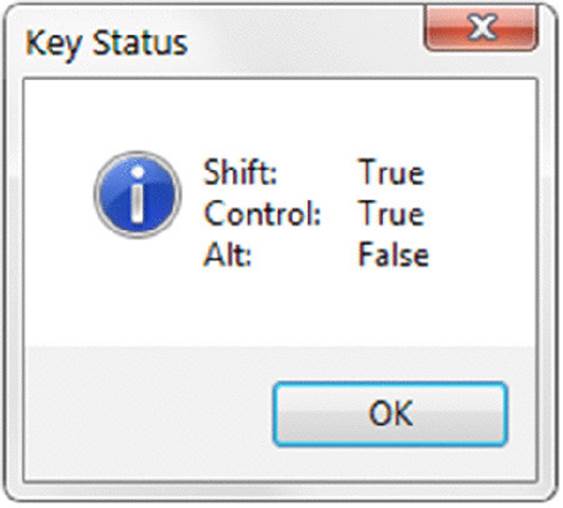
Figure 5.11 Using Windows API functions to determine which keys were pressed.

Learning more about API functions

Working with the Windows API functions can be tricky. Many programming reference books list the declarations for common API calls and often provide examples. Usually, you can simply copy the declarations and use the functions without understanding the details. Many Excel programmers take a cookbook approach to API functions. The Internet has dozens of reliable examples that you can copy and paste. Or search the web for a file named Win32API_PtrSafe.txt. This file, from Microsoft, contains many examples of declaration statements.

Cross-Ref

Chapter 7 has several additional examples of using Windows API functions.