Excel 2016 Power Programming with VBA (2016)
Part I. Introduction to Excel VBA
Chapter 7. VBA Programming Examples and Techniques
In This Chapter
· Using VBA to work with ranges
· Using VBA to work with workbooks and sheets
· Creating custom functions for use in your VBA procedures and in worksheet formulas
· Trying miscellaneous VBA tricks and techniques
· Using Windows Application Programming Interface (API) functions
Learning by Example
Most beginning VBA programmers benefit from hands-on examples. A well-thought-out example usually communicates a concept much better than a description of the underlying theory. Therefore, instead of taking you through a painful review of every nuance of VBA, this chapter guides you through demonstrations of useful Excel programming techniques.
Here, you will walk through examples that solve practical problems while furthering your knowledge of VBA. This includes:
· Working with ranges
· Working with workbooks and sheets
· VBA techniques
· Functions that are useful in your VBA procedures
· Functions that you can use in worksheet formulas
· Windows API calls
 Cross-Ref
Subsequent chapters in this book present additional feature-specific examples: charts, pivot tables, events, UserForms, and so on.
Working with Ranges
The examples in this section demonstrate how to manipulate worksheet ranges with VBA.
Specifically, we provide examples of copying a range, moving a range, selecting a range, identifying types of information in a range, prompting for a cell value, determining the first empty cell in a column, pausing a macro to allow the user to select a range, counting cells in a range, looping through the cells in a range, and several other commonly used range-related operations.
Copying a range
Excel’s macro recorder is useful not so much for generating usable code but for discovering the names of relevant objects, methods, and properties. The code that’s generated by the macro recorder isn’t always the most efficient, but it can usually provide you with several clues.
For example, recording a simple copy-and-paste operation generates five lines of VBA code:
Sub Macro1()
Range("A1").Select
Selection.Copy
Range("B1").Select
ActiveSheet.Paste
Application.CutCopyMode = False
End Sub
Note that the generated code selects cell A1, copies it, and then selects cell B1 and performs the paste operation. But in VBA, you don’t need to select an object to work with it. You would never learn this important point by mimicking the preceding recorded macro code, where two statements incorporate the Select method. You can replace this procedure with the following much simpler routine, which doesn’t select any cells. It also takes advantage of the fact that the Copy method can use an argument that represents the destination for the copied range.
Sub CopyRange()
Range("A1").Copy Range("B1")
End Sub
Both macros assume that a worksheet is active and that the operation takes place on the active worksheet. To copy a range to a different worksheet or workbook, simply qualify the range reference for the destination. The following example copies a range from Sheet1in File1.xlsx to Sheet2 in File2.xlsx. Because the references are fully qualified, this example works regardless of which workbook is active.
Sub CopyRange2()
Workbooks("File1.xlsx").Sheets("Sheet1").Range("A1").Copy _
Workbooks("File2.xlsx").Sheets("Sheet2").Range("A1")
End Sub
Another way to approach this task is to use object variables to represent the ranges, as shown in the code that follows. Using object variables is especially useful when your code will use the ranges at some other point.
Sub CopyRange3()
Dim Rng1 As Range, Rng2 As Range
Set Rng1 = Workbooks("File1.xlsx").Sheets("Sheet1").Range("A1")
Set Rng2 = Workbooks("File2.xlsx").Sheets("Sheet2").Range("A1")
Rng1.Copy Rng2
End Sub
As you might expect, copying isn’t limited to one single cell at a time. The following procedure, for example, copies a large range. Note that the destination consists of only a single cell (which represents the upper-left cell for the destination). Using a single cell for the destination works just like it does when you copy and paste a range manually in Excel.
Sub CopyRange4()
Range("A1:C800").Copy Range("D1")
End Sub
Moving a range
The VBA instructions for moving a range are similar to those for copying a range, as the following example demonstrates. The difference is that you use the Cut method instead of the Copy method. Note that you need to specify only the upper-left cell for the destination range.
The following example moves 18 cells (in A1:C6) to a new location, beginning at cell H1:
Sub MoveRange1()
Range("A1:C6").Cut Range("H1")
End Sub
Copying a variably sized range
In many cases, you need to copy a range of cells, but you don’t know the exact row and column dimensions of the range. For example, you might have a workbook that tracks weekly sales, and the number of rows changes weekly when you add new data.
Figure 7.1 shows a common type of worksheet. This range consists of several rows, and the number of rows changes each week. Because you don’t know the exact range address at any given time, writing a macro to copy the range requires additional coding.
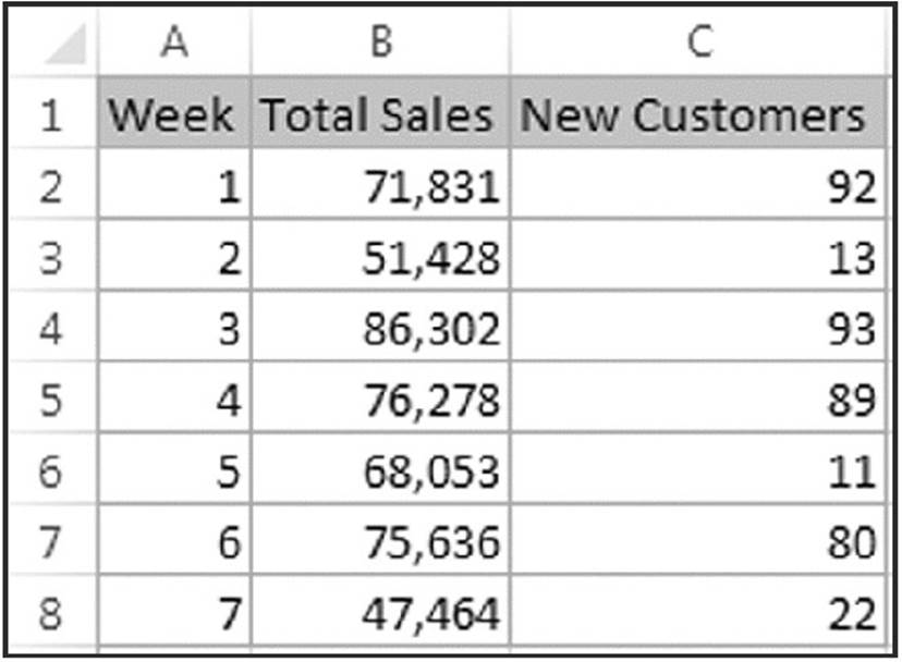
Figure 7.1 The number of rows in the data range changes every week.
The following macro demonstrates how to copy this range from Sheet1 to Sheet2 (beginning at cell A1). It uses the CurrentRegion property, which returns a Range object that corresponds to the block of cells around a particular cell (in this case, A1).
Sub CopyCurrentRegion2()
Range("A1").CurrentRegion.Copy Sheets("Sheet2").Range("A1")
End Sub
 Note
Note
Using the CurrentRegion property is equivalent to choosing the Home ➜ Editing ➜ Find & Select ➜ Go To Special command and selecting the Current Region option (or by using the Ctrl+Shift+* shortcut to select the current region). To see how theCurrentRegion selection works, record your actions while you issue that command. Generally, the CurrentRegion property setting consists of a rectangular block of cells surrounded by one or more blank rows or columns.
If the range to be copied is a table (specified by choosing Insert ➜ Tables ➜ Table), you can use code like this (assuming the table is named Table1):
Sub CopyTable()
Range("Table1[#All]").Copy Sheets("Sheet2").Range("A1")
End Sub
 Tips for working with ranges
When you work with ranges, keep the following points in mind:
· Your code doesn’t need to select a range to work with it.
· You can’t select a range that’s not on the active worksheet. So if your code does select a range, its worksheet must be active. You can use the Activate method of the Worksheets collection to activate a particular sheet.
· Remember that the macro recorder doesn’t always generate the most efficient code. Often, you can create your macro by using the recorder and then edit the code to make it more efficient.
· Using named ranges in your VBA code is a good idea. For example, refer to Range("Total") rather than Range("D45"). In the latter case, if you add a row above row 45, the cell address will change. You would then need to modify the macro so that it uses the correct range address (D46).
· If you rely on the macro recorder when selecting ranges, make sure that you record the macro using relative references. Choose Developer ➜ Code ➜ Use Relative References to toggle this setting.
· When running a macro that works on each cell in the current range selection, the user might select entire columns or rows. In most cases, you don’t want to loop through every cell in the selection. Your macro should create a subset of the selection consisting of only the nonblank cells. See the section “Looping through a selected range efficiently,” later in this chapter.
· Excel allows multiple selections. For example, you can select a range, press Ctrl, and select another range. You can test for multiple selections in your macro and take appropriate action. See the section “Determining the type of selected range,” later in this chapter.
Selecting or otherwise identifying various types of ranges
Much of the work that you’ll do in VBA will involve working with ranges — either selecting a range or identifying a range so that you can do something with the cells.
In addition to the CurrentRegion property (which we discussed earlier), you should also be aware of the End method of the Range object. The End method takes one argument, which determines the direction in which the selection is extended. The following statement selects a range from the active cell to the last nonempty cell in that column:
Range(ActiveCell, ActiveCell.End(xlDown)).Select
Here’s a similar example that uses a specific cell as the starting point:
Range(Range("A2"), Range("A2").End(xlDown)).Select
As you might expect, three other constants simulate key combinations in the other directions: xlUp, xlToLeft, and xlToRight.
 Caution
Be careful when using the End method with the ActiveCell property. If the active cell is at the perimeter of a range or if the range contains one or more empty cells, the End method may not produce the desired results.
 On the Web
This book’s website includes a workbook that demonstrates several common types of range selections. When you open this workbook, named range selections.xlsm, the code adds a new menu item to the shortcut menu that appears when you right-click a cell: Selection Demo. This menu contains commands that enable the user to make various types of selections, as shown in Figure 7.2.
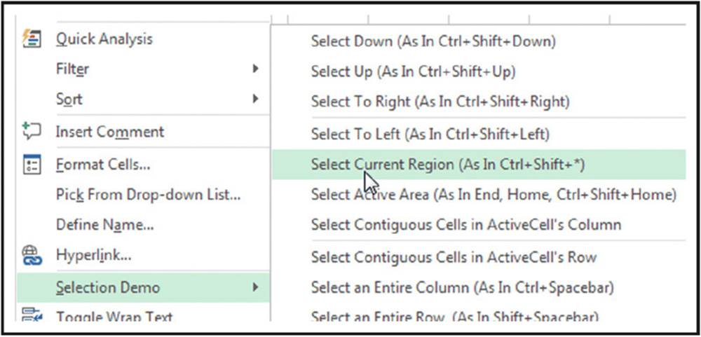
Figure 7.2 This workbook uses a custom shortcut menu to demonstrate how to select variably sized ranges by using VBA.
The following macro is in the example workbook. The SelectCurrentRegion macro simulates pressing Ctrl+Shift+*.
Sub SelectCurrentRegion()
ActiveCell.CurrentRegion.Select
End Sub
Often, you won’t want to select the cells. Rather, you’ll want to work with them in some way (for example, format them). You can easily adapt the cell-selecting procedures. The following procedure was adapted from SelectCurrentRegion. This procedure doesn’t select cells; it applies formatting to the range defined as the current region around the active cell. You can adapt the other procedures in the example workbook in this manner.
Sub FormatCurrentRegion()
ActiveCell.CurrentRegion.Font.Bold = True
End Sub
Another way to refer to a range
If you look at VBA code written by others, you may notice a different way to reference a range. For example, the following statement selects a range:
[C2:D8].Select
The range address is surrounded by square brackets, and the range address is not enclosed in quote marks. The preceding statement is equivalent to:
Range("C2:D8").Select
Using square brackets is a shortcut for the Evaluate method of the Application object. In this example, it’s a shortcut for:
Application.Evaluate("C2:D8").Select
This may save a few keystrokes when entering the code, but it ends up being a bit slower than the normal type of referencing because it takes time to evaluate a text string and determine that it’s a range reference.
Resizing a range
The Resize property of a Range object makes it easy to change the size of a range. The Resize property takes two arguments that represent the total number of rows and the total number of columns in the resized range.
For example, after executing the following statement, the MyRange object variable is 20 rows by 5 columns (range A1:E20):
Set MyRange = Range("A1")
Set MyRange = MyRange.Resize(20, 5)
After the following statement is executed, the size of MyRange is increased by one row. Note that the second argument is omitted, so the number of columns does not change.
Set MyRange = MyRange.Resize(MyRange.Rows.Count + 1)
A more practical example involves changing the definition of a range name. Assume a workbook has a range named Data. Your code needs to extend the named range by adding an additional row. This code snippet will do the job:
With Range("Data")
.Resize(.Rows.Count + 1).Name ="Data"
End With
Prompting for a cell value
The following procedure demonstrates how to ask the user for a value and then insert it into cell A1 of the active worksheet:
Sub GetValue1()
Range("A1").Value = InputBox("Enter the value")
End Sub
Figure 7.3 shows how the input box looks.
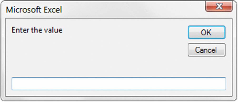
Figure 7.3 The InputBox function gets a value from the user to be inserted into a cell.
This procedure has a problem, however. If the user clicks the Cancel button in the input box, the procedure deletes any data already in the cell. The following modification takes no action if the Cancel button is clicked (which results in an empty string for the UserEntryvariable):
Sub GetValue2()
Dim UserEntry As Variant
UserEntry = InputBox("Enter the value")
If UserEntry <>"" Then Range("A1").Value = UserEntry
End Sub
In many cases, you’ll need to validate the user’s entry in the input box. For example, you may require a number between 1 and 12. The following example demonstrates one way to validate the user’s entry. In this example, an invalid entry is ignored, and the input box is displayed again. This cycle keeps repeating until the user enters a valid number or clicks Cancel.
Sub GetValue3()
Dim UserEntry As Variant
Dim Msg As String
Const MinVal As Integer = 1
Const MaxVal As Integer = 12
Msg ="Enter a value between" & MinVal &" and" & MaxVal
Do
UserEntry = InputBox(Msg)
If UserEntry ="" Then Exit Sub
If IsNumeric(UserEntry) Then
If UserEntry >= MinVal And UserEntry <= MaxVal Then Exit Do
End If
Msg ="Your previous entry was INVALID."
Msg = Msg & vbNewLine
Msg = Msg &"Enter a value between" & MinVal &" and" & MaxVal
Loop
ActiveSheet.Range("A1").Value = UserEntry
End Sub
As you can see in Figure 7.4, the code also changes the message displayed if the user makes an invalid entry.
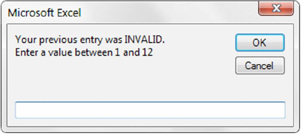
Figure 7.4 Validate a user’s entry with the VBA InputBox function.
On the Web
The three GetValue procedures are available on this book’s website in the inputbox demo.xlsm file.
Entering a value in the next empty cell
A common requirement is to enter a value into the next empty cell in a column or row. The following example prompts the user for a name and a value and then enters the data into the next empty row (see Figure 7.5).
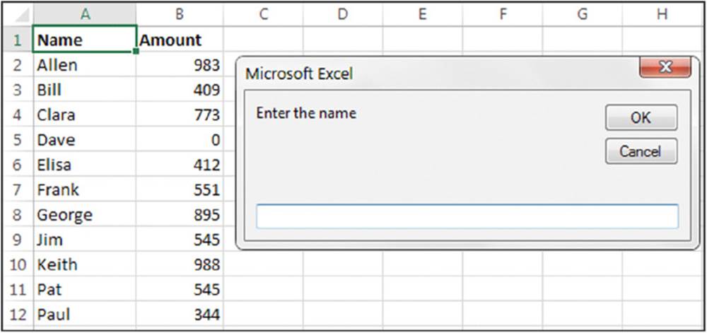
Figure 7.5 A macro for inserting data into the next empty row in a worksheet.
Sub GetData()
Dim NextRow As Long
Dim Entry1 As String, Entry2 As String
Do
'Determine next empty row
NextRow = Cells(Rows.Count, 1).End(xlUp).Row + 1
' Prompt for the data
Entry1 = InputBox("Enter the name")
If Entry1 ="" Then Exit Sub
Entry2 = InputBox("Enter the amount")
If Entry2 ="" Then Exit Sub
' Write the data
Cells(NextRow, 1) = Entry1
Cells(NextRow, 2) = Entry2
Loop
End Sub
To keep things simple, this procedure doesn’t perform any validation. The loop continues indefinitely. We use Exit Sub statements to get out of the loop when the user clicks Cancel in the input box.
On the Web
The GetData procedure is available on the book’s website in the next empty cell.xlsm file.
Note the statement that determines the value of the NextRow variable. If you don’t understand how this statement works, try the manual equivalent: Activate the last cell in column A (cell A1048576), press End, and then press the up-arrow key. At this point, the last nonblank cell in column A will be selected. The Row property returns this row number, which is incremented by 1 to get the row of the cell below it (the next empty row). Rather than hard-code the last cell in column A, we used Rows.Count so that this procedure will be compatible with all versions of Excel (including versions before Excel 2007 where the rows on a worksheet were capped at 65,536).
This technique of selecting the next empty cell has a slight glitch. If the column is empty, it will calculate row 2 as the next empty row. Writing additional code to account for this possibility would be fairly easy.
Pausing a macro to get a user-selected range
In some situations, you may need an interactive macro. For example, you can create a macro that pauses while the user specifies a range of cells. The procedure in this section describes how to do this with Excel’s InputBox method.
Note
Don’t confuse Excel’s InputBox method with VBA’s InputBox function. Although these two items have the same name, they’re not the same.
The Sub procedure that follows demonstrates how to pause a macro and let the user select a range. The code then inserts a formula in each cell of the specified range.
Sub GetUserRange()
Dim UserRange As Range
Prompt ="Select a range for the random numbers."
Title ="Select a range"
' Display the Input Box
On Error Resume Next
Set UserRange = Application.InputBox( _
Prompt:=Prompt, _
Title:=Title, _
Default:=ActiveCell.Address, _
Type:=8) 'Range selection
On Error GoTo 0
' Was the Input Box canceled?
If UserRange Is Nothing Then
MsgBox"Canceled."
Else
UserRange.Formula ="=RAND()"
End If
End Sub
The input box is shown in Figure 7.6.
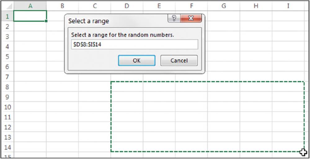
Figure 7.6 Use an input box to pause a macro.
On the Web
This example, named prompt for a range.xlsm, is available on this book’s website.
Specifying a Type argument of 8 for the InputBox method is the key to this procedure. Type argument 8 tells Excel that the input box should only accept a valid range.
Also note the use of On Error Resume Next. This statement ignores the error that occurs if the user clicks the Cancel button. If the user clicks Cancel, the UserRange object variable isn’t defined. This example displays a message box with the text Canceled. If the user clicks OK, the macro continues. Using On Error GoTo 0 resumes normal error handling.
By the way, you don’t need to check for a valid range selection. Excel takes care of this task for you. If the user types an invalid range address, Excel displays a message box with instructions on how to select a range.
Counting selected cells
You can create a macro that works with the range of cells selected by the user. Use the Count property of the Range object to determine how many cells are contained in a range selection (or any range, for that matter). For example, the following statement displays a message box that contains the number of cells in the current selection:
MsgBox Selection.Count
Caution
With the larger worksheet size introduced in Excel 2007, the Count property can generate an error. The Count property uses the Long data type, so the largest value that it can store is 2,147,483,647. For example, if the user selects 2,048 complete columns (2,147,483,648 cells), the Count property generates an error. Fortunately, Microsoft added a new property beginning with Excel 2007: CountLarge. CountLarge uses the Double data type, which can handle values up to 1.79+E^308.
The bottom line? In the vast majority of situations, the Count property will work fine. If there’s a chance that you may need to count more cells (such as all cells in a worksheet), use CountLarge instead of Count.
If the active sheet contains a range named Data, the following statement assigns the number of cells in the Data range to a variable named CellCount:
CellCount = Range("Data").Count
You can also determine how many rows or columns are contained in a range. The following expression calculates the number of columns in the currently selected range:
Selection.Columns.Count
And, of course, you can use the Rows property to determine the number of rows in a range. The following statement counts the number of rows in a range named Data and assigns the number to a variable named RowCount:
RowCount = Range("Data").Rows.Count
Determining the type of selected range
Excel supports several types of range selections:
· A single cell
· A contiguous range of cells
· One or more entire columns
· One or more entire rows
· The entire worksheet
· Any combination of the preceding (that is, a multiple selection)
As a result, when your VBA procedure processes a user-selected range, you can’t make any presumptions about what that range might be. For example, the range selection might consist of two areas, say A1:A10 and C1:C10. (To make a multiple selection, press Ctrl while you select the ranges with your mouse.)
In the case of a multiple range selection, the Range object comprises separate areas. To determine whether a selection is a multiple selection, use the Areas method, which returns an Areas collection. This collection represents all the ranges in a multiple range selection.
You can use an expression such as the following to determine whether a selected range has multiple areas:
NumAreas = Selection.Areas.Count
If the NumAreas variable contains a value greater than 1, the selection is a multiple selection.
Following is a function named AreaType, which returns a text string that describes the type of range selection:
Function AreaType(RangeArea As Range) As String
' Returns the type of a range in an area
Select Case True
Case RangeArea.Cells.CountLarge = 1
AreaType ="Cell"
Case RangeArea.CountLarge = Cells.CountLarge
AreaType ="Worksheet"
Case RangeArea.Rows.Count = Cells.Rows.Count
AreaType ="Column"
Case RangeArea.Columns.Count = Cells.Columns.Count
AreaType ="Row"
Case Else
AreaType ="Block"
End Select
End Function
This function accepts a Range object as its argument and returns one of five strings that describe the area: Cell, Worksheet, Column, Row, or Block. The function uses a Select Case construct to determine which of five comparison expressions is True. For example, if the range consists of a single cell, the function returns Cell. If the number of cells in the range is equal to the number of cells in the worksheet, it returns Worksheet. If the number of rows in the range equals the number of rows in the worksheet, it returns Column. If the number of columns in the range equals the number of columns in the worksheet, the function returns Row. If none of the Case expressions is True, the function returns Block.
Note that we used the CountLarge property when counting cells. As we noted previously in this chapter, the number of selected cells could potentially exceed the limit of the Count property.
On the Web
This example is available on this book’s website in a file named about range selection.xlsm. The workbook contains a procedure (named RangeDescription) that uses the AreaType function to display a message box that describes the current range selection.Figure 7.7 shows an example. Understanding how this routine works will give you a good foundation for working with Range objects.
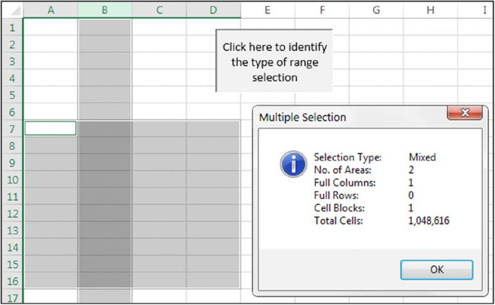
Figure 7.7 A VBA procedure analyzes the currently selected range.
Note
You might be surprised to discover that Excel allows multiple selections to be identical. For example, if you hold down Ctrl and click five times in cell A1, the selection will have five identical areas. The RangeDescription procedure takes this possibility into account and doesn’t count the same cell multiple times. Also note that Excel displays progressively darker shading for overlapping range selections.
Looping through a selected range efficiently
A common task is to create a macro that evaluates each cell in a range and performs an operation if the cell meets a certain criterion. The procedure that follows is an example of such a macro. The ColorNegative procedure sets the cell’s background color to red for cells that contain a negative value. For non-negative value cells, it sets the background color to none.
Note
This example is for educational purposes only. Using Excel’s conditional formatting feature is a much better approach.
Sub ColorNegative()
' Makes negative cells red
Dim cell As Range
If TypeName(Selection) <>"Range" Then Exit Sub
Application.ScreenUpdating = False
For Each cell In Selection
If cell.Value < 0 Then
cell.Interior.Color = RGB(255, 0, 0)
Else
cell.Interior.Color = xlNone
End If
Next cell
End Sub
The ColorNegative procedure certainly works, but it has a serious flaw. For example, what if the used area on the worksheet were small, but the user selects an entire column? Or ten columns? Or the entire worksheet? You don’t need to process all those empty cells, and the user would probably give up long before your code churns through all those cells.
A better solution (ColorNegative2) follows. In this revised procedure, we create a Range object variable, WorkRange, which consists of the intersection of the user’s selected range and the worksheet’s used range.
Sub ColorNegative2()
' Makes negative cells red
Dim WorkRange As Range
Dim cell As Range
If TypeName(Selection) <>"Range" Then Exit Sub
Application.ScreenUpdating = False
Set WorkRange = Application.Intersect(Selection, ActiveSheet.UsedRange)
For Each cell In WorkRange
If cell.Value < 0 Then
cell.Interior.Color = RGB(255, 0, 0)
Else
cell.Interior.Color = xlNone
End If
Next cell
End Sub
Figure 7.8 shows an example; the entire column D is selected (1,048,576 cells). The range used by the worksheet, however, is B2:I16. Therefore, the intersection of these ranges is D2:D16, which is a much smaller range than the original selection. Needless to say, the time difference between processing 15 cells versus processing 1,048,576 cells is significant.
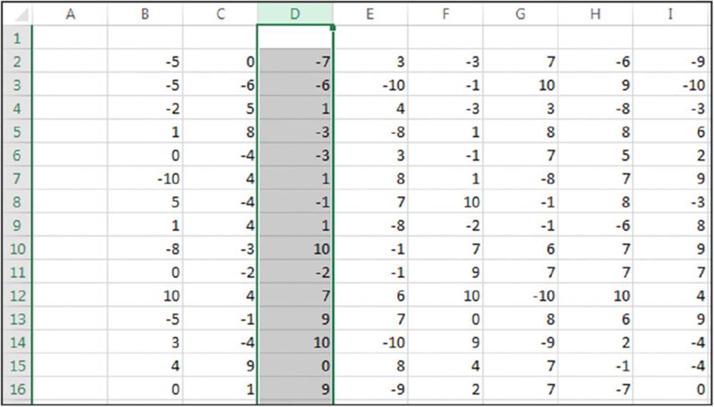
Figure 7.8 Using the intersection of the used range and the selected range results in fewer cells to process.
The ColorNegative2 procedure is an improvement, but it’s still not as efficient as it could be because it processes empty cells. A third revision, ColorNegative3, is quite a bit longer but much more efficient. We use the SpecialCells method to generate two subsets of the selection: One subset (ConstantCells) includes only the cells with numeric constants; the other subset (FormulaCells) includes only the cells with numeric formulas. The code processes the cells in these subsets by using two For Each-Next constructs. The net effect: Only nonblank, nontext cells are evaluated, thus speeding up the macro considerably.
Sub ColorNegative3()
' Makes negative cells red
Dim FormulaCells As Range, ConstantCells As Range
Dim cell As Range
If TypeName(Selection) <>"Range" Then Exit Sub
Application.ScreenUpdating = False
' Create subsets of original selection
On Error Resume Next
Set FormulaCells = Selection.SpecialCells(xlFormulas, xlNumbers)
Set ConstantCells = Selection.SpecialCells(xlConstants, xlNumbers)
On Error GoTo 0
' Process the formula cells
If Not FormulaCells Is Nothing Then
For Each cell In FormulaCells
If cell.Value < 0 Then
cell.Interior.Color = RGB(255, 0, 0)
Else
cell.Interior.Color = xlNone
End If
Next cell
End If
' Process the constant cells
If Not ConstantCells Is Nothing Then
For Each cell In ConstantCells
If cell.Value < 0 Then
cell.Interior.Color = RGB(255, 0, 0)
Else
cell.Interior.Color = xlNone
End If
Next cell
End If
End Sub
Note
The On Error statement is necessary because the SpecialCells method generates an error if no cells qualify.
On the Web
A workbook that contains the three ColorNegative procedures is available on this book’s website in the efficient looping.xlsm file.
Deleting all empty rows
The following procedure deletes all empty rows in the active worksheet. This routine is fast and efficient because it doesn’t check all rows. It checks only the rows in the used range, which is determined by using the UsedRange property of the Worksheet object.
Sub DeleteEmptyRows()
Dim LastRow As Long
Dim r As Long
Dim Counter As Long
Application.ScreenUpdating = False
LastRow = ActiveSheet.UsedRange.Rows.Count+ActiveSheet.UsedRange.Rows(1).Row-1
For r = LastRow To 1 Step -1
If Application.WorksheetFunction.CountA(Rows(r)) = 0 Then
Rows(r).Delete
Counter = Counter + 1
End If
Next r
Application.ScreenUpdating = True
MsgBox Counter &" empty rows were deleted."
End Sub
The first step is to determine the last used row and then assign this row number to the LastRow variable. This calculation isn’t as simple as you might think because the used range may or may not begin in row 1. Therefore, LastRow is calculated by determining the number of rows in the used range, adding the first row number in the used range, and subtracting 1.
The procedure uses Excel’s COUNTA worksheet function to determine whether a row is empty. If this function returns 0 for a particular row, the row is empty. Note that the procedure works on the rows from bottom to top and also uses a negative step value in theFor-Next loop. This negative step value is necessary because deleting rows causes all subsequent rows to move up in the worksheet. If the looping occurred from top to bottom, the counter in the loop wouldn’t be accurate after a row is deleted.
The macro uses another variable, Counter, to keep track of how many rows were deleted. This number is displayed in a message box when the procedure ends.
On the Web
A workbook that contains this example is available on this book’s website in a file named delete empty rows.xlsm.
Duplicating rows a variable number of times
The example in this section demonstrates how to use VBA to create duplicates of a row. Figure 7.9 shows a worksheet for an office raffle. Column A contains the name, and column B contains the number of tickets purchased by each person. Column C contains a random number (generated by the RAND function). The winner will be determined by sorting the data based on column C (the highest random number wins).
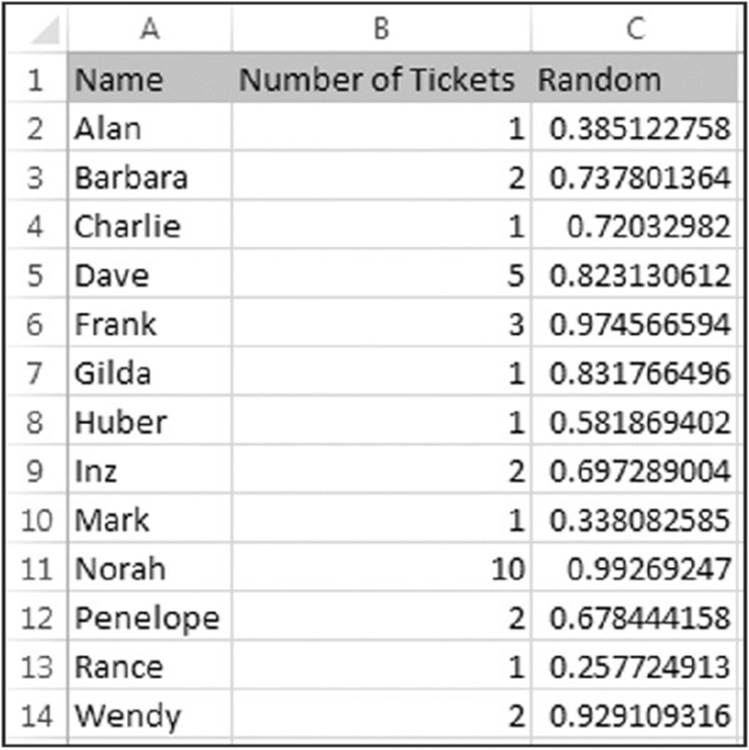
Figure 7.9 The goal is to duplicate rows based on the value in column B.
The macro duplicates the rows so that each person will have a row for each ticket purchased. For example, Barbara purchased two tickets, so she should have two rows (and two chances to win).
The procedure to insert the new rows is shown here:
Sub DupeRows()
Dim cell As Range
' First cell with number of tickets
Set cell = Range("B2")
Do While Not IsEmpty(cell)
If cell > 1 Then
Range(cell.Offset(1, 0), cell.Offset(cell.Value - 1, _
0)).EntireRow.Insert
Range(cell, cell.Offset(cell.Value - 1, 1)).EntireRow.FillDown
End If
Set cell = cell.Offset(cell.Value, 0)
Loop
End Sub
The cell object variable is initialized to cell B2, the first cell that has a number. The loop inserts new rows and then copies the row using the FillDown method. The cell variable is incremented to the next person, and the loop continues until an empty cell is encountered. Figure 7.10 shows a portion of the worksheet after running this procedure.
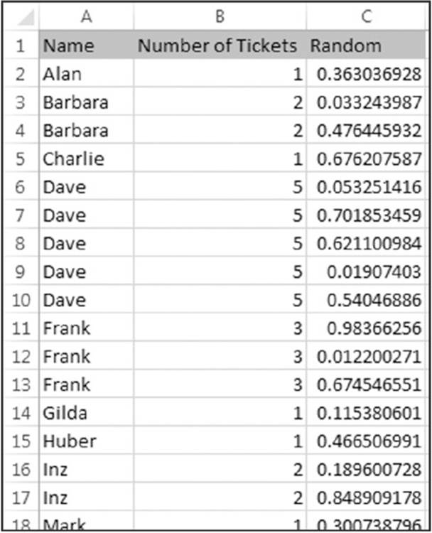
Figure 7.10 New rows were added, according to the value in column B.
On the Web
A workbook that contains this example is available on this book’s website in the duplicate rows.xlsm file.
Determining whether a range is contained in another range
The following InRange function accepts two arguments, both Range objects. The function returns True if the first range is contained in the second range. This function can be used in a worksheet formula, but it’s more useful when called by another procedure.
Function InRange(rng1, rng2) As Boolean
' Returns True if rng1 is a subset of rng2
On Error GoTo ErrHandler
If Union(rng1, rng2).Address = rng2.Address Then
InRange = True
Exit Function
End If
ErrHandler:
InRange = False
End Function
The Union method of the Application object returns a Range object that represents the union of two Range objects. The union consists of all the cells from both ranges. If the address of the union of the two ranges is the same as the address of the second range, the first range is contained in the second range.
If the two ranges are in different worksheets, the Union method generates an error. The On Error statement handles this situation.
On the Web
A workbook that contains this function is available on this book’s website in the inrange function.xlsm file.
Determining a cell’s data type
Excel provides a number of built-in functions that can help determine the type of data contained in a cell. Examples of these functions are ISTEXT, ISLOGICAL, and ISERROR. In addition, VBA includes functions such as IsEmpty, IsDate, and IsNumeric.
The following function, named CellType, accepts a range argument and returns a string (Blank, Text, Logical, Error, Date, Time, or Number) that describes the data type of the upper-left cell in the range.
Function CellType(Rng) As String
' Returns the cell type of the upper left cell in a range
Dim TheCell As Range
Set TheCell = Rng.Range("A1")
Select Case True
Case IsEmpty(TheCell)
CELLTYPE ="Blank"
Case TheCell.NumberFormat ="@"
CELLTYPE ="Text"
Case Application.IsText(TheCell)
CELLTYPE ="Text"
Case Application.IsLogical(TheCell)
CELLTYPE ="Logical"
Case Application.IsErr(TheCell)
CELLTYPE ="Error"
Case IsDate(TheCell)
CELLTYPE ="Date"
Case InStr(1, TheCell.Text,":") <> 0
CELLTYPE ="Time"
Case IsNumeric(TheCell)
CELLTYPE ="Number"
End Select
End Function
You can use this function in a worksheet formula or from another VBA procedure. In Figure 7.11, the function is used in formulas in column B. These formulas use data in column A as the argument. Column C is just a description of the data.
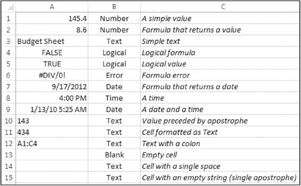
Figure 7.11 Using a function to determine the type of data in a cell.
Note the use of the Set TheCell statement. The CellType function accepts a range argument of any size, but this statement causes it to operate on only the upper-left cell in the range (which is represented by the TheCell variable).
On the Web
A workbook that contains this function is available on this book’s website in the celltype function.xlsm file.
Reading and writing ranges
Many VBA tasks involve transferring values either from an array to a range or from a range to an array. Excel reads from ranges much faster than it writes to ranges because (presumably) the latter operation involves the calculation engine. The WriteReadRangeprocedure that follows demonstrates the relative speeds of writing and reading a range.
This procedure creates an array and then uses For-Next loops to write the array to a range and then read the range back into the array. It calculates the time required for each operation by using the VBA Timer function.
Sub WriteReadRange()
Dim MyArray()
Dim Time1 As Double
Dim NumElements As Long, i As Long
Dim WriteTime As String, ReadTime As String
Dim Msg As String
NumElements = 250000
ReDim MyArray(1 To NumElements)
' Fill the array
For i = 1 To NumElements
MyArray(i) = i
Next i
' Write the array to a range
Time1 = Timer
For i = 1 To NumElements
Cells(i, 1) = MyArray(i)
Next i
WriteTime = Format(Timer - Time1,"00:00")
' Read the range into the array
Time1 = Timer
For i = 1 To NumElements
MyArray(i) = Cells(i, 1)
Next i
ReadTime = Format(Timer - Time1,"00:00")
' Show results
Msg ="Write:" & WriteTime
Msg = Msg & vbCrLf
Msg = Msg &"Read:" & ReadTime
MsgBox Msg, vbOKOnly, NumElements &" Elements"
End Sub
The results of the timed test will be presented in the form of a message box telling you how long it took to write and read 250,000 elements to and from an array (see Figure 7.12).
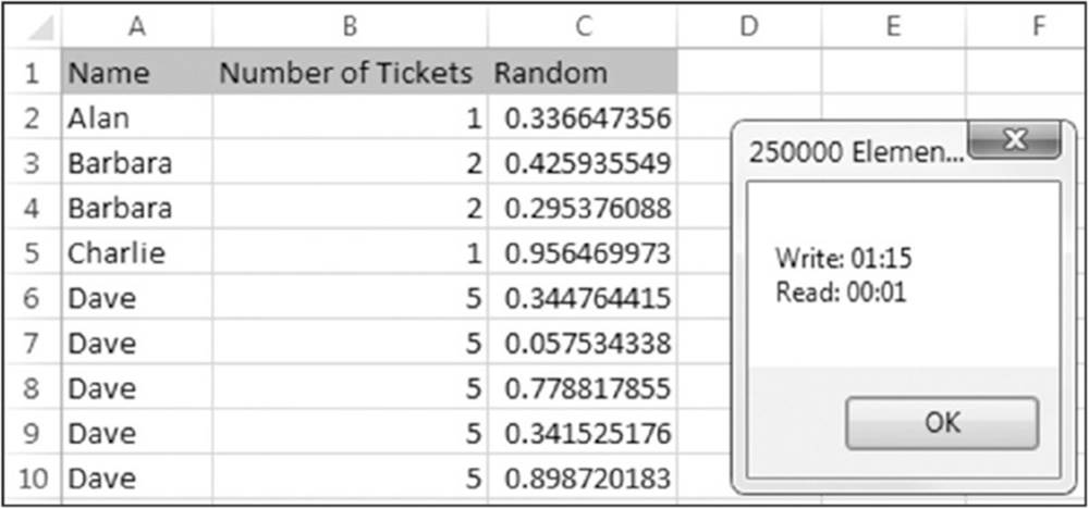
Figure 7.12 Displaying the time to write to a range and read from a range, using a loop.
A better way to write to a range
The example in the preceding section uses a For-Next loop to transfer the contents of an array to a worksheet range. In this section, we demonstrate a more efficient way to accomplish this task.
Start with the example that follows, which illustrates the most obvious (but not the most efficient) way to fill a range. This example uses a For-Next loop to insert its values in a range.
Sub LoopFillRange()
' Fill a range by looping through cells
Dim CellsDown As Long, CellsAcross As Integer
Dim CurrRow As Long, CurrCol As Integer
Dim StartTime As Double
Dim CurrVal As Long
' Get the dimensions
CellsDown = InputBox("How many cells down?")
If CellsDown = 0 Then Exit Sub
CellsAcross = InputBox("How many cells across?")
If CellsAcross = 0 Then Exit Sub
' Record starting time
StartTime = Timer
' Loop through cells and insert values
CurrVal = 1
Application.ScreenUpdating = False
For CurrRow = 1 To CellsDown
For CurrCol = 1 To CellsAcross
ActiveCell.Offset(CurrRow - 1, _
CurrCol - 1).Value = CurrVal
CurrVal = CurrVal + 1
Next CurrCol
Next CurrRow
' Display elapsed time
Application.ScreenUpdating = True
MsgBox Format(Timer - StartTime,"00.00") &" seconds"
End Sub
The example that follows demonstrates a much faster way to produce the same result. This code inserts the values into an array and then uses a single statement to transfer the contents of an array to the range.
Sub ArrayFillRange()
' Fill a range by transferring an array
Dim CellsDown As Long, CellsAcross As Integer
Dim i As Long, j As Integer
Dim StartTime As Double
Dim TempArray() As Long
Dim TheRange As Range
Dim CurrVal As Long
' Get the dimensions
CellsDown = InputBox("How many cells down?")
If CellsDown = 0 Then Exit Sub
CellsAcross = InputBox("How many cells across?")
If CellsAcross = 0 Then Exit Sub
' Record starting time
StartTime = Timer
' Redimension temporary array
ReDim TempArray(1 To CellsDown, 1 To CellsAcross)
' Set worksheet range
Set TheRange = ActiveCell.Range(Cells(1, 1), _
Cells(CellsDown, CellsAcross))
' Fill the temporary array
CurrVal = 0
Application.ScreenUpdating = False
For i = 1 To CellsDown
For j = 1 To CellsAcross
TempArray(i, j) = CurrVal + 1
CurrVal = CurrVal + 1
Next j
Next i
' Transfer temporary array to worksheet
TheRange.Value = TempArray
' Display elapsed time
Application.ScreenUpdating = True
MsgBox Format(Timer - StartTime,"00.00") &" seconds"
End Sub
On my system, using the loop method to fill a 1000 x 250–cell range (250,000 cells) took 15.80 seconds. The array transfer method took only 0.15 seconds to generate the same results — more than 100 times faster! The moral of this story? If you need to transfer large amounts of data to a worksheet, avoid looping whenever possible.
Note
The timing results are highly dependent on the presence of formulas. Generally, you’ll get faster transfer times if no workbooks are open that contain formulas or if you set the calculation mode to Manual.
On the Web
A workbook that contains the WriteReadRange, LoopFillRange, and ArrayFillRange procedures is available on this book’s website. The file is named loop vs array fill range.xlsm.
Transferring one-dimensional arrays
The example in the preceding section involves a two-dimensional array, which works out nicely for row-and-column-based worksheets.
When transferring a one-dimensional array to a range, the range must be horizontal — that is, one row with multiple columns. If you need the data in a vertical range instead, you must first transpose the array to make it vertical. You can use Excel’s TRANSPOSE function to do this. The following example transfers a 100-element array to a vertical worksheet range (A1:A100):
Range("A1:A100").Value = Application.WorksheetFunction.Transpose(MyArray)
Transferring a range to a variant array
This section discusses yet another way to work with worksheet data in VBA. The following example transfers a range of cells to a two-dimensional variant array. Then message boxes display the upper bounds for each dimension of the variant array.
Sub RangeToVariant()
Dim x As Variant
x = Range("A1:L600").Value
MsgBox UBound(x, 1)
MsgBox UBound(x, 2)
End Sub
In this example, the first message box displays 600 (the number of rows in the original range), and the second message box displays 12 (the number of columns). You’ll find that transferring the range data to a variant array is virtually instantaneous.
The following example reads a range (named data) into a variant array, performs a simple multiplication operation on each element in the array, and then transfers the variant array back to the range:
Sub RangeToVariant2()
Dim x As Variant
Dim r As Long, c As Integer
' Read the data into the variant
x = Range("data").Value
' Loop through the variant array
For r = 1 To UBound(x, 1)
For c = 1 To UBound(x, 2)
' Multiply by 2
x(r, c) = x(r, c) * 2
Next c
Next r
' Transfer the variant back to the sheet
Range("data") = x
End Sub
You’ll find that this procedure runs amazingly fast. Working with 30,000 cells took less than 1 second.
On the Web
A workbook that contains this example is available on this book’s website in the variant transfer.xlsm file.
Selecting cells by value
The example in this section demonstrates how to select cells based on their value. Oddly, Excel doesn’t provide a direct way to perform this operation. The SelectByValue procedure follows. In this example, the code selects cells that contain a negative value, but you can easily change the code to select cells based on other criteria.
Sub SelectByValue()
Dim Cell As Object
Dim FoundCells As Range
Dim WorkRange As Range
If TypeName(Selection) <>"Range" Then Exit Sub
' Check all or selection?
If Selection.CountLarge = 1 Then
Set WorkRange = ActiveSheet.UsedRange
Else
Set WorkRange = Application.Intersect(Selection, ActiveSheet.UsedRange)
End If
' Reduce the search to numeric cells only
On Error Resume Next
Set WorkRange = WorkRange.SpecialCells(xlConstants, xlNumbers)
If WorkRange Is Nothing Then Exit Sub
On Error GoTo 0
' Loop through each cell, add to the FoundCells range if it qualifies
For Each Cell In WorkRange
If Cell.Value < 0 Then
If FoundCells Is Nothing Then
Set FoundCells = Cell
Else
Set FoundCells = Union(FoundCells, Cell)
End If
End If
Next Cell
' Show message, or select the cells
If FoundCells Is Nothing Then
MsgBox"No cells qualify."
Else
FoundCells.Select
MsgBox"Selected" & FoundCells.Count &" cells."
End If
End Sub
The procedure starts by checking the selection. If it’s a single cell, the entire worksheet is searched. If the selection is at least two cells, only the selected range is searched. The range to be searched is further refined by using the SpecialCells method to create a Rangeobject that consists only of the numeric constants.
The code in the For-Next loop examines the cell’s value. If it meets the criterion (less than 0), the cell is added to the FoundCells Range object by using the Union method. Note that you can’t use the Union method for the first cell. If the FoundCells range contains no cells, attempting to use the Union method will generate an error. Therefore, the code checks whether FoundCells is Nothing.
When the loop ends, the FoundCells object will consist of the cells that meet the criterion (or will be Nothing if no cells were found). If no cells are found, a message box appears. Otherwise, the cells are selected.
On the Web
This example is available on this book’s website in the select by value.xlsm file.
Copying a noncontiguous range
If you’ve ever attempted to copy a noncontiguous range selection, you discovered that Excel doesn’t support such an operation. Attempting to do so displays the following error message: That command cannot be used on multiple selections.
An exception is when you attempt to copy a multiple selection that consists of entire rows or columns, or when the multiple selections are in the same row(s) or same column(s). Excel does allow those operations. But when you paste the copied cells, all blanks are removed.
When you encounter a limitation in Excel, you can often circumvent it by creating a macro. The example in this section is a VBA procedure that allows you to copy a multiple selection to another location.
Sub CopyMultipleSelection()
Dim SelAreas() As Range
Dim PasteRange As Range
Dim UpperLeft As Range
Dim NumAreas As Long, i As Long
Dim TopRow As Long, LeftCol As Long
Dim RowOffset As Long, ColOffset As Long
If TypeName(Selection) <>"Range" Then Exit Sub
' Store the areas as separate Range objects
NumAreas = Selection.Areas.Count
ReDim SelAreas(1 To NumAreas)
For i = 1 To NumAreas
Set SelAreas(i) = Selection.Areas(i)
Next
' Determine the upper-left cell in the multiple selection
TopRow = ActiveSheet.Rows.Count
LeftCol = ActiveSheet.Columns.Count
For i = 1 To NumAreas
If SelAreas(i).Row < TopRow Then TopRow = SelAreas(i).Row
If SelAreas(i).Column < LeftCol Then LeftCol = SelAreas(i).Column
Next
Set UpperLeft = Cells(TopRow, LeftCol)
' Get the paste address
On Error Resume Next
Set PasteRange = Application.InputBox _
(Prompt:="Specify the upper-left cell for the paste range:", _
Title:="Copy Multiple Selection", _
Type:=8)
On Error GoTo 0
' Exit if canceled
If TypeName(PasteRange) <>"Range" Then Exit Sub
' Make sure only the upper-left cell is used
Set PasteRange = PasteRange.Range("A1")
' Copy and paste each area
For i = 1 To NumAreas
RowOffset = SelAreas(i).Row - TopRow
ColOffset = SelAreas(i).Column - LeftCol
SelAreas(i).Copy PasteRange.Offset(RowOffset, ColOffset)
Next i
End Sub
Figure 7.13 shows the prompt to select the destination location.
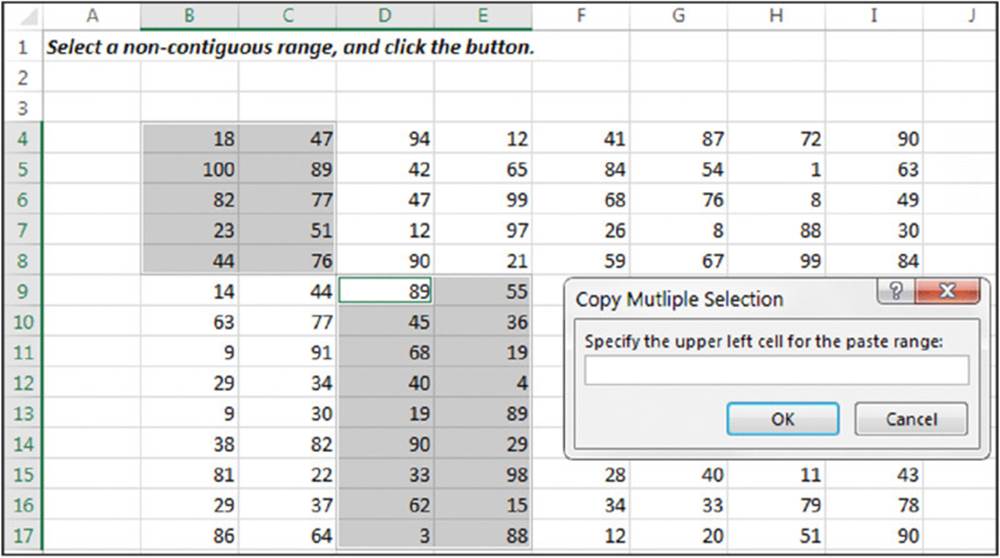
Figure 7.13 Using Excel’s InputBox method to prompt for a cell location.
On the Web
This book’s website contains a workbook with this example, plus another version that warns the user if data will be overwritten. The file is named copy multiple selection.xlsm.
Working with Workbooks and Sheets
The examples in this section demonstrate various ways to use VBA to work with workbooks and worksheets.
Saving all workbooks
The following procedure loops through all workbooks in the Workbooks collection and saves each file that has been saved previously:
Public Sub SaveAllWorkbooks()
Dim Book As Workbook
For Each Book In Workbooks
If Book.Path <>"" Then Book.Save
Next Book
End Sub
Note the use of the Path property. If a workbook’s Path property is empty, the file has never been saved (it’s a newly created workbook). This procedure ignores such workbooks and saves only the workbooks that have a nonempty Path property.
A more efficient approach also checks the Saved property. This property is True if the workbook has not been changed since it was last saved. The SaveAllWorkbooks2 procedure doesn’t save files that don’t need to be saved.
Public Sub SaveAllWorkbooks2()
Dim Book As Workbook
For Each Book In Workbooks
If Book.Path <>"" Then
If Book.Saved <> True Then
Book.Save
End If
End If
Next Book
End Sub
Saving and closing all workbooks
The following procedure loops through the Workbooks collection. The code saves and closes all workbooks.
Sub CloseAllWorkbooks()
Dim Book As Workbook
For Each Book In Workbooks
If Book.Name <> ThisWorkbook.Name Then
Book.Close savechanges:=True
End If
Next Book
ThisWorkbook.Close savechanges:=True
End Sub
The procedure uses an If statement in the For-Next loop to determine whether the workbook is the workbook that contains the code. This statement is necessary because closing the workbook that contains the procedure would end the code, and subsequent workbooks wouldn’t be affected. After all the other workbooks are closed, the workbook that contains the code closes itself.
Hiding all but the selection
The example in this section hides all rows and columns in a worksheet except those in the current range selection:
Sub HideRowsAndColumns()
Dim row1 As Long, row2 As Long
Dim col1 As Long, col2 As Long
If TypeName(Selection) <>"Range" Then Exit Sub
' If last row or last column is hidden, unhide all and quit
If Rows(Rows.Count).EntireRow.Hidden Or _
Columns(Columns.Count).EntireColumn.Hidden Then
Cells.EntireColumn.Hidden = False
Cells.EntireRow.Hidden = False
Exit Sub
End If
row1 = Selection.Rows(1).Row
row2 = row1 + Selection.Rows.Count - 1
col1 = Selection.Columns(1).Column
col2 = col1 + Selection.Columns.Count - 1
Application.ScreenUpdating = False
On Error Resume Next
' Hide rows
Range(Cells(1, 1), Cells(row1 - 1, 1)).EntireRow.Hidden = True
Range(Cells(row2 + 1, 1), Cells(Rows.Count, 1)).EntireRow.Hidden = True
' Hide columns
Range(Cells(1, 1), Cells(1, col1 - 1)).EntireColumn.Hidden = True
Range(Cells(1, col2 + 1), Cells(1, Columns.Count)).EntireColumn.Hidden = True
End Sub
Figure 7.14 shows an example. If the range selection consists of a noncontiguous range, the first area is used as the basis for hiding rows and columns. Note that it’s a toggle. Executing the procedures when the last row or last column is hidden unhides all rows and columns.
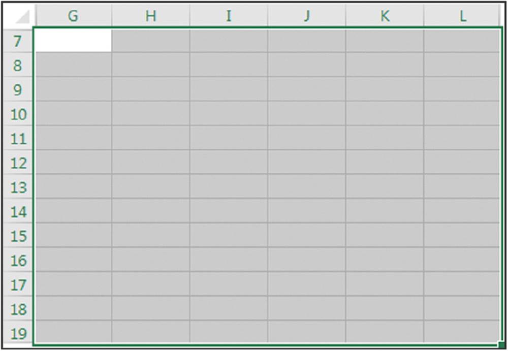
Figure 7.14 All rows and columns are hidden, except for a range (G7:L19).
On the Web
A workbook with this example is available on this book’s website in the hide rows and columns.xlsm file.
Creating a hyperlink table of contents
The CreateTOC procedure inserts a new worksheet at the beginning of the active workbook. It then creates a table of contents, in the form of a list of hyperlinks to each worksheet.
Sub CreateTOC()
Dim i As Integer
Sheets.Add Before:=Sheets(1)
For i = 2 To Worksheets.Count
ActiveSheet.Hyperlinks.Add _
Anchor:=Cells(i, 1), _
Address:="", _
SubAddress:="'" & Worksheets(i).Name &"'!A1", _
TextToDisplay:=Worksheets(i).Name
Next i
End Sub
It’s not possible to create a hyperlink to a chart sheet, so the code uses the Worksheet collection rather than the Sheets collection.
Figure 7.15 shows an example of a hyperlink table of contents that contains worksheets comprised of month names.
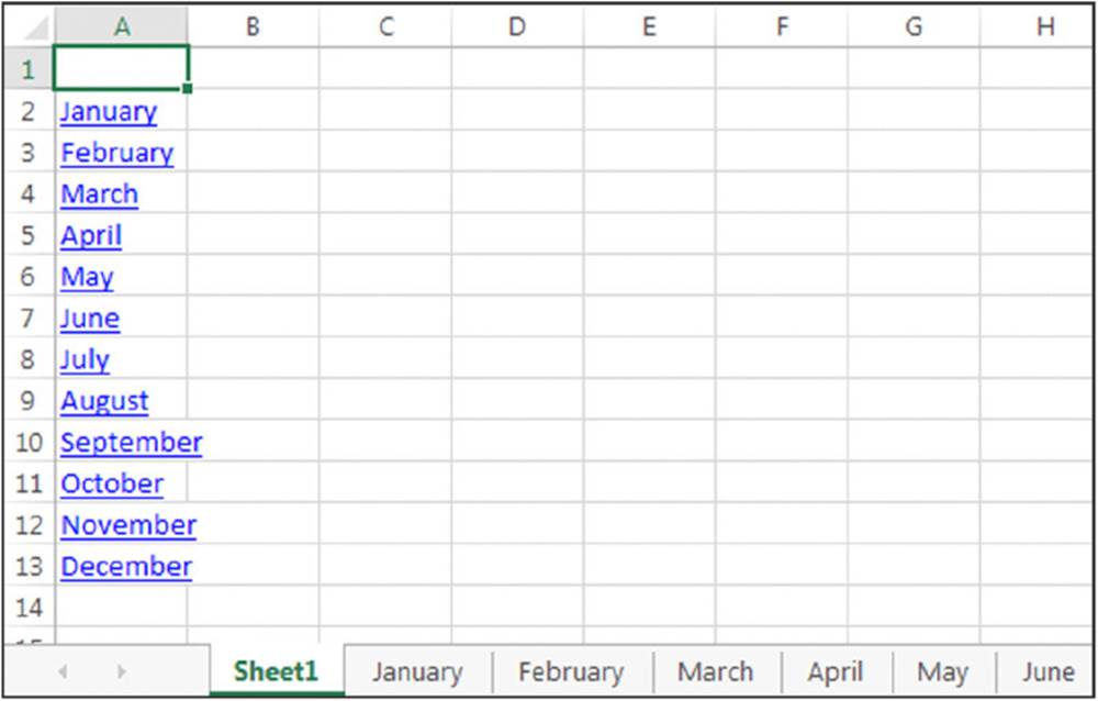
Figure 7.15 Hyperlinks to each worksheet, created by a macro.
On the Web
A workbook with this example is available on this book’s website in the create hyperlinks.xlsm file.
Synchronizing worksheets
If you use multisheet workbooks, you probably know that Excel can’t synchronize the sheets in a workbook. In other words, there is no automatic way to force all sheets to have the same selected range and upper-left cell. The VBA macro that follows uses the active worksheet as a base and then performs the following on all other worksheets in the workbook:
· Selects the same range as the active sheet
· Makes the upper-left cell the same as the active sheet
Following is the listing for the procedure:
Sub SynchSheets()
' Duplicates the active sheet's active cell and upper left cell
' Across all worksheets
If TypeName(ActiveSheet) <>"Worksheet" Then Exit Sub
Dim UserSheet As Worksheet, sht As Worksheet
Dim TopRow As Long, LeftCol As Integer
Dim UserSel As String
Application.ScreenUpdating = False
' Remember the current sheet
Set UserSheet = ActiveSheet
' Store info from the active sheet
TopRow = ActiveWindow.ScrollRow
LeftCol = ActiveWindow.ScrollColumn
UserSel = ActiveWindow.RangeSelection.Address
' Loop through the worksheets
For Each sht In ActiveWorkbook.Worksheets
If sht.Visible Then 'skip hidden sheets
sht.Activate
Range(UserSel).Select
ActiveWindow.ScrollRow = TopRow
ActiveWindow.ScrollColumn = LeftCol
End If
Next sht
' Restore the original position
UserSheet.Activate
Application.ScreenUpdating = True
End Sub
On the Web
A workbook with this example is available on this book’s website in the synchronize sheets.xlsm file.
VBA Techniques
The examples in this section illustrate common VBA techniques that you might be able to adapt to your own projects.
Toggling a Boolean property
A Boolean property is one that is either True or False. The easiest way to toggle a Boolean property is to use the Not operator, as shown in the following example, which toggles the WrapText property of a selection:
Sub ToggleWrapText()
' Toggles text wrap alignment for selected cells
If TypeName(Selection) ="Range" Then
Selection.WrapText = Not ActiveCell.WrapText
End If
End Sub
You can modify this procedure to toggle other Boolean properties.
Note that the active cell is used as the basis for toggling. When a range is selected and the property values in the cells are inconsistent (for example, some cells are bold and others are not), Excel uses the active cell to determine how to toggle. If the active cell is bold, for example, all cells in the selection are made not bold when you click the Bold button. This simple procedure mimics the way Excel works, which is usually the best practice.
Note also that this procedure uses the TypeName function to check whether the selection is a range. If the selection isn’t a range, nothing happens.
You can use the Not operator to toggle many other properties. For example, to toggle the display of row and column borders in a worksheet, use the following code:
ActiveWindow.DisplayHeadings = Not ActiveWindow.DisplayHeadings
To toggle the display of gridlines in the active worksheet, use the following code:
ActiveWindow.DisplayGridlines = Not ActiveWindow.DisplayGridlines
Displaying the date and time
If you understand the serial number system that Excel uses to store dates and times, you won’t have any problems using dates and times in your VBA procedures.
The DateAndTime procedure displays a message box with the current date and time, as depicted in Figure 7.16. This example also displays a personalized message in the message box’s title bar.
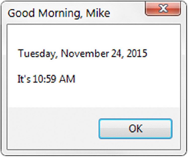
Figure 7.16 A message box displaying the date and time.
The procedure uses the Date function as an argument for the Format function. The result is a string with a nicely formatted date. We used the same technique to get a nicely formatted time.
Sub DateAndTime()
Dim TheDate As String, TheTime As String
Dim Greeting As String
Dim FullName As String, FirstName As String
Dim SpaceInName As Long
TheDate = Format(Date,"Long Date")
TheTime = Format(Time,"Medium Time")
' Determine greeting based on time
Select Case Time
Case Is < TimeValue("12:00"): Greeting ="Good Morning,"
Case Is >= TimeValue("17:00"): Greeting ="Good Evening,"
Case Else: Greeting ="Good Afternoon,"
End Select
' Append user's first name to greeting
FullName = Application.UserName
SpaceInName = InStr(1, FullName,"", 1)
' Handle situation when name has no space
If SpaceInName = 0 Then SpaceInName = Len(FullName)
FirstName = Left(FullName, SpaceInName)
Greeting = Greeting & FirstName
' Show the message
MsgBox TheDate & vbCrLf & vbCrLf &"It's" & TheTime, vbOKOnly, Greeting
End Sub
In the preceding example, we used named formats (Long Date and Medium Time) to ensure that the macro will work properly regardless of the user’s international settings. You can, however, use other formats. For example, to display the date in mm/dd/yy format, you can use a statement like the following:
TheDate = Format(Date,"mm/dd/yy")
We used a Select Case construct to base the greeting displayed in the message box’s title bar on the time of day. VBA time values work just as they do in Excel. If the time is less than .5 (noon), it’s morning. If it’s greater than .7083 (5 p.m.), it’s evening. Otherwise, it’s afternoon. We took the easy way out and used VBA’s TimeValue function, which returns a time value from a string.
The next series of statements determines the user’s first name, as recorded in the General tab in Excel’s Options dialog box. We used the VBA InStr function to locate the first space in the user’s name. The MsgBox function concatenates the date and time but uses the built-in vbCrLf constant to insert a line break between them. vbOKOnly is a predefined constant that returns 0, causing the message box to appear with only an OK button. The final argument is the Greeting, constructed earlier in the procedure.
On the Web
The DateAndTime procedure is available on this book’s website, in a file named date and time.xlsm.
Displaying friendly time
If you’re not a stickler for 100 percent accuracy, you might like the FT function, listed here. FT, which stands for friendly time, displays a time difference in words.
Function FT(t1, t2)
Dim SDif As Double, DDif As Double
If Not (IsDate(t1) And IsDate(t2)) Then
FT = CVErr(xlErrValue)
Exit Function
End If
DDif = Abs(t2 - t1)
SDif = DDif * 24 * 60 * 60
If DDif < 1 Then
If SDif < 10 Then FT ="Just now": Exit Function
If SDif < 60 Then FT = SDif &" seconds ago": Exit Function
If SDif < 120 Then FT ="a minute ago": Exit Function
If SDif < 3600 Then FT = Round(SDif / 60, 0) &"minutes ago": Exit Function
If SDif < 7200 Then FT ="An hour ago": Exit Function
If SDif < 86400 Then FT = Round(SDif / 3600, 0) &" hours ago": Exit Function
End If
If DDif = 1 Then FT ="Yesterday": Exit Function
If DDif < 7 Then FT = Round(DDif, 0) &" days ago": Exit Function
If DDif < 31 Then FT = Round(DDif / 7, 0) &" weeks ago": Exit Function
If DDif < 365 Then FT = Round(DDif / 30, 0) &" months ago": Exit Function
FT = Round(DDif / 365, 0) &" years ago"
End Function
Figure 7.17 shows examples of this function used in formulas. If you actually have a need for such a way to display time differences, this procedure leaves lots of room for improvement. For example, you can write code to prevent displays such as 1 months ago and 1 years ago.
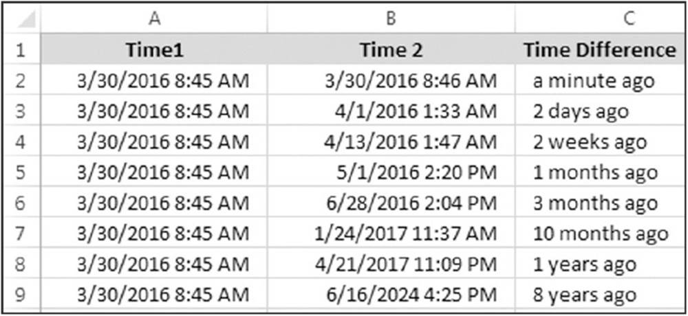
Figure 7.17 Using a function to display time differences in a friendly manner.
On the Web
This example is available on this book’s website. The file is named friendly time .xlsm.
Getting a list of fonts
If you need to get a list of all installed fonts, you’ll find that Excel doesn’t provide a direct way to retrieve that information. The technique described here takes advantage of the fact that Excel still supports the old CommandBar properties and methods for compatibility with pre–Excel 2007 versions. These properties and methods were used to work with toolbars and menus.
The ShowInstalledFonts macro displays a list of the installed fonts in column A of the active worksheet. It creates a temporary toolbar (a CommandBar object), adds the Font control, and reads the font names from that control. The temporary toolbar is then deleted.
Sub ShowInstalledFonts()
Dim FontList As CommandBarControl
Dim TempBar As CommandBar
Dim i As Long
' Create temporary CommandBar
Set TempBar = Application.CommandBars.Add
Set FontList = TempBar.Controls.Add(ID:=1728)
' Put the fonts into column A
Range("A:A").ClearContents
For i = 0 To FontList.ListCount - 1
Cells(i + 1, 1) = FontList.List(i + 1)
Next i
' Delete temporary CommandBar
TempBar.Delete
End Sub
 Tip
Tip
As an option, you can display each font name in the actual font (as shown in Figure 7.18). To do so, add this statement inside the For-Next loop:
Cells(i+1,1).Font.Name = FontList.List(i+1)
Be aware, however, that using many fonts in a workbook can eat up lots of system resources and could even crash your system.
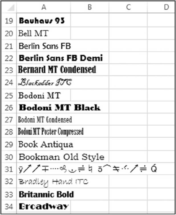
Figure 7.18 Listing font names in the actual fonts.
On the Web
This procedure is available on the book’s website in the list fonts.xlsm file.
Sorting an array
Although Excel has a built-in command to sort worksheet ranges, VBA doesn’t offer a method to sort arrays. One viable (but cumbersome) workaround is to transfer your array to a worksheet range, sort it by using Excel’s commands, and then return the result to your array. This method is surprisingly fast, but if you need something faster, use a sorting routine written in VBA.
In this section, we cover four different sorting techniques:
· Worksheet sort transfers an array to a worksheet range, sorts it, and transfers it back to the array. This procedure accepts an array as its only argument.
· Bubble sort is a simple sorting technique (also used in the Chapter 4 sheet-sorting example). Although easy to program, the bubble-sorting algorithm tends to be slow, especially with many elements.
· Quick sort is a much faster sorting routine than bubble sort, but it is also more difficult to understand. This technique works only with Integer and Long data types.
· Counting sort is lightning fast but difficult to understand. Like the quick sort, this technique works only with Integer and Long data types.
On the Web
The book’s website includes a workbook application that demonstrates these sorting methods. This workbook, named sorting demo.xlsm, is useful for comparing these techniques with arrays of varying sizes. However, you can also copy the procedures and use them in your code.
The worksheet sort algorithm is amazingly fast, especially when you consider that the array is transferred to the sheet, sorted, and then transferred back to the array.
The bubble sort algorithm is the simplest and is reasonably fast with small arrays, but for larger arrays (more than 10,000 elements), forget it. The quick sort and counting sort algorithms are blazingly fast, but they’re limited to Integer and Long data types.
Figure 7.19 shows the dialog box for this project.
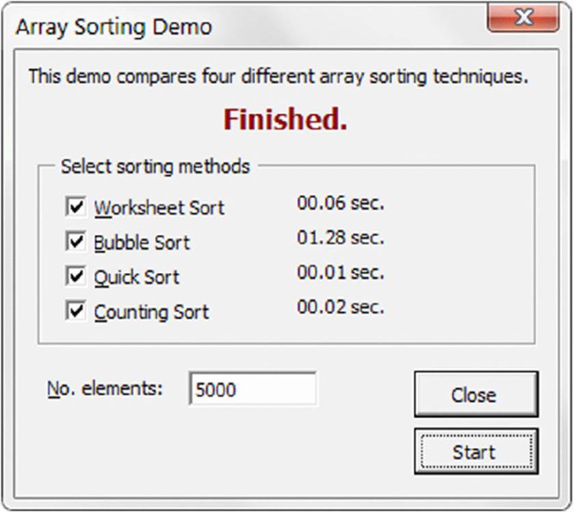
Figure 7.19 Comparing the time required to perform sorts of various array sizes.
Processing a series of files
One common use for macros is to perform repetitive tasks. The example in this section demonstrates how to execute a macro that operates on several different files stored on disk. This example, which may help you set up your own routine for this type of task, prompts the user for a file specification and then processes all matching files. In this case, processing consists of importing the file and entering a series of summary formulas that describe the data in the file.
Sub BatchProcess()
Dim FileSpec As String
Dim i As Integer
Dim FileName As String
Dim FileList() As String
Dim FoundFiles As Integer
' Specify path and file spec
FileSpec = ThisWorkbook.Path &"\" &"text??.txt"
FileName = Dir(FileSpec)
' Was a file found?
If FileName <>"" Then
FoundFiles = 1
ReDim Preserve FileList(1 To FoundFiles)
FileList(FoundFiles) = FileName
Else
MsgBox"No files were found that match" & FileSpec
Exit Sub
End If
' Get other filenames
Do
FileName = Dir
If FileName ="" Then Exit Do
FoundFiles = FoundFiles + 1
ReDim Preserve FileList(1 To FoundFiles)
FileList(FoundFiles) = FileName &"*"
Loop
' Loop through the files and process them
For i = 1 To FoundFiles
Call ProcessFiles(FileList(i))
Next i
End Sub
On the Web
This example, named batch processing.xlsm, is available on the book’s website. It uses three additional files (also available for download): text01.txt, text02 .txt, and text03.txt. You’ll need to modify the routine to import other text files.
The matching filenames are stored in an array named FoundFiles, and the procedure uses a For-Next loop to process the files. Within the loop, the processing is done by calling the ProcessFiles procedure, which follows. This simple procedure uses the OpenText method to import the file and then inserts five formulas. You may, of course, substitute your own routine in place of this one:
Sub ProcessFiles(FileName As String)
' Import the file
Workbooks.OpenText FileName:=FileName, _
Origin:=xlWindows, _
StartRow:=1, _
DataType:=xlFixedWidth, _
FieldInfo:= _
Array(Array(0, 1), Array(3, 1), Array(12, 1))
' Enter summary formulas
Range("D1").Value ="A"
Range("D2").Value ="B"
Range("D3").Value ="C"
Range("E1:E3").Formula ="=COUNTIF(B:B,D1)"
Range("F1:F3").Formula ="=SUMIF(B:B,D1,C:C)"
End Sub
Cross-Ref
For more information about working with files using VBA, refer to Chapter 11.
Some Useful Functions for Use in Your Code
In this section, we present some custom utility functions that you may find useful in your own applications and that may provide inspiration for creating similar functions. These functions are most useful when called from another VBA procedure. Therefore, they’re declared by using the Private keyword so that they won’t appear in Excel’s Insert Function dialog box.
On the Web
The examples in this section are available on the book’s website in the VBA utility functions.xlsm file.
The FileExists function
The FileExists function takes one argument (a path with a filename) and returns True if the file exists:
Private Function FileExists(fname) As Boolean
' Returns TRUE if the file exists
FileExists = (Dir(fname) <>"")
End Function
The FileNameOnly function
The FileNameOnly function accepts one argument (a path with a filename) and returns only the filename. In other words, it strips out the path.
Private Function FileNameOnly(pname) As String
' Returns the filename from a path/filename string
Dim temp As Variant
length = Len(pname)
temp = Split(pname, Application.PathSeparator)
FileNameOnly = temp(UBound(temp))
End Function
The function uses the VBA Split function, which accepts a string (that includes delimiter characters), and returns a variant array that contains the elements between the delimiter characters. In this case the temp variable contains an array that consists of each text string between the Application.PathSeparater (usually a backslash character). For another example of the Split function, see the section"Extracting the nth element from a string," later in this chapter.
If the argument is c:\excel files\2016\backup\budget.xlsx, the function returns the string budget.xlsx.
The FileNameOnly function works with any path and filename (even if the file does not exist). If the file exists, the following function is a simpler way to strip the path and return only the filename:
Private Function FileNameOnly2(pname) As String
FileNameOnly2 = Dir(pname)
End Function
The PathExists function
The PathExists function accepts one argument (a path) and returns True if the path exists:
Private Function PathExists(pname) As Boolean
' Returns TRUE if the path exists
If Dir(pname, vbDirectory) ="" Then
PathExists = False
Else
PathExists = (GetAttr(pname) And vbDirectory) = vbDirectory
End If
End Function
The RangeNameExists function
The RangeNameExists function accepts a single argument (a range name) and returns True if the range name exists in the active workbook:
Private Function RangeNameExists(nname) As Boolean
' Returns TRUE if the range name exists
Dim n As Name
RangeNameExists = False
For Each n In ActiveWorkbook.Names
If UCase(n.Name) = UCase(nname) Then
RangeNameExists = True
Exit Function
End If
Next n
End Function
Another way to write this function follows. This version attempts to create an object variable using the name. If doing so generates an error, the name doesn’t exist.
Private Function RangeNameExists2(nname) As Boolean
' Returns TRUE if the range name exists
Dim n As Range
On Error Resume Next
Set n = Range(nname)
If Err.Number = 0 Then RangeNameExists2 = True _
Else RangeNameExists2 = False
End Function
The SheetExists function
The SheetExists function accepts one argument (a worksheet name) and returns True if the worksheet exists in the active workbook:
Private Function SheetExists(sname) As Boolean
' Returns TRUE if sheet exists in the active workbook
Dim x As Object
On Error Resume Next
Set x = ActiveWorkbook.Sheets(sname)
If Err.Number = 0 Then SheetExists = True Else SheetExists = False
End Function
The WorkbookIsOpen function
The WorkbookIsOpen function accepts one argument (a workbook name) and returns True if the workbook is open:
Private Function WorkbookIsOpen(wbname) As Boolean
' Returns TRUE if the workbook is open
Dim x As Workbook
On Error Resume Next
Set x = Workbooks(wbname)
If Err.Number = 0 Then WorkbookIsOpen = True _
Else WorkbookIsOpen = False
End Function
Testing for membership in a collection
The following function procedure is a generic function that you can use to determine whether an object is a member of a collection:
Private Function IsInCollection_
(Coln As Object, Item As String) As Boolean
Dim Obj As Object
On Error Resume Next
Set Obj = Coln(Item)
IsInCollection = Not Obj Is Nothing
End Function
This function accepts two arguments: the collection (an object) and the item (a string) that might or might not be a member of the collection. The function attempts to create an object variable that represents the item in the collection. If the attempt is successful, the function returns True; otherwise, it returns False.
You can use the IsInCollection function in place of three other functions listed in this chapter: RangeNameExists, SheetExists, and WorkbookIsOpen. To determine whether a range named Data exists in the active workbook, call the IsInCollection function with this statement:
MsgBox IsInCollection(ActiveWorkbook.Names,"Data")
To determine whether a workbook named Budget is open, use this statement:
MsgBox IsInCollection(Workbooks,"budget.xlsx")
To determine whether the active workbook contains a sheet named Sheet1, use this statement:
MsgBox IsInCollection(ActiveWorkbook.Worksheets,"Sheet1")
Retrieving a value from a closed workbook
VBA doesn’t include a method to retrieve a value from a closed workbook file. You can, however, take advantage of Excel’s capability to work with linked files. This section contains a custom VBA function (GetValue, which follows) that retrieves a value from a closed workbook. It does so by calling an XLM macro, which is an old-style macro used in versions before Excel 5. Fortunately, Excel still supports this old macro system.
Private Function GetValue(path, file, sheet, ref)
' Retrieves a value from a closed workbook
Dim arg As String
' Make sure the file exists
If Right(path, 1) <>"\" Then path = path &"\"
If Dir(path & file) ="" Then
GetValue ="File Not Found"
Exit Function
End If
' Create the argument
arg ="'" & path &"[" & file &"]" & sheet &"'!" & _
Range(ref).Range("A1").Address(, , xlR1C1)
' Execute an XLM macro
GetValue = ExecuteExcel4Macro(arg)
End Function
The GetValue function takes four arguments:
· path: The drive and path to the closed file (for example,"d:\files")
· file: The workbook name (for example,"budget.xlsx")
· sheet: The worksheet name (for example,"Sheet1")
· ref: The cell reference (for example,"C4")
The following Sub procedure demonstrates how to use the GetValue function. It displays the value in cell A1 in Sheet1 of a file named 2013budget.xlsx, located in the XLFiles\Budget directory on drive C.
Sub TestGetValue()
Dim p As String, f As String
Dim s As String, a As String
p ="c:\XLFiles\Budget"
f ="2013budget.xlsx"
s ="Sheet1"
a ="A1"
MsgBox GetValue(p, f, s, a)
End Sub
Another example follows. This procedure reads 1,200 values (100 rows and 12 columns) from a closed file and then places the values into the active worksheet.
Sub TestGetValue2()
Dim p As String, f As String
Dim s As String, a As String
Dim r As Long, c As Long
p ="c:\XLFiles\Budget"
f ="2013Budget.xlsx"
s ="Sheet1"
Application.ScreenUpdating = False
For r = 1 To 100
For c = 1 To 12
a = Cells(r, c).Address
Cells(r, c) = GetValue(p, f, s, a)
Next c
Next r
End Sub
An alternative is to write code that turns off screen updating, opens the file, gets the value, and then closes the file. Unless the file is very large, the user won’t even notice that a file is being opened.
Note
The GetValue function doesn’t work in a worksheet formula. However, there is no need to use this function in a formula. You can simply create a link formula to retrieve a value from a closed file.
On the Web
This example is available on this book’s website in the value from a closed workbook.xlsm file. The example uses a file named myworkbook.xlsx for the closed file.
Some Useful Worksheet Functions
The examples in this section are custom functions that you can use in worksheet formulas. Remember, you must define these Function procedures in a VBA module (not a code module associated with ThisWorkbook, a Sheet, or a UserForm).
On the Web
The examples in this section are available on the book’s website in the worksheet functions.xlsm file.
Returning cell formatting information
This section contains a number of custom functions that return information about a cell’s formatting. These functions are useful if you need to sort data based on formatting (for example, sort in such a way that all bold cells are together).
Caution
You’ll find that these functions aren’t always updated automatically because changing formatting doesn’t trigger Excel’s recalculation engine. To force a global recalculation (and update all custom functions), press Ctrl+Alt+F9.
Alternatively, you can add the following statement to your function:
Application.Volatile
When this statement is present, pressing F9 will recalculate the function.
The following function returns TRUE if its single-cell argument has bold formatting. If a range is passed as the argument, the function uses the upper-left cell of the range.
Function ISBOLD(cell) As Boolean
' Returns TRUE if cell is bold
ISBOLD = cell.Range("A1").Font.Bold
End Function
Note that this function works only with explicitly applied formatting. It doesn’t work for formatting applied using conditional formatting. Excel 2010 introduced DisplayFormat, a new object that takes conditional formatting into account. Here’s the ISBOLD function rewritten so that it works also with bold formatting applied as a result of conditional formatting:
Function ISBOLD (cell) As Boolean
' Returns TRUE if cell is bold, even if from conditional formatting
ISBOLD = cell.Range("A1").DisplayFormat.Font.Bold
End Function
The following function returns TRUE if its single-cell argument has italic formatting:
Function ISITALIC(cell) As Boolean
' Returns TRUE if cell is italic
ISITALIC = cell.Range("A1").Font.Italic
End Function
Both functions will return an error if the cell has mixed formatting — for example, if only some characters are bold. The following function returns TRUE only if all characters in the cell are bold:
Function ALLBOLD(cell) As Boolean
' Returns TRUE if all characters in cell are bold
If IsNull(cell.Font.Bold) Then
ALLBOLD = False
Else
ALLBOLD = cell.Font.Bold
End If
End Function
You can simplify the ALLBOLD function as follows:
Function ALLBOLD (cell) As Boolean
' Returns TRUE if all characters in cell are bold
ALLBOLD = Not IsNull(cell.Font.Bold)
End Function
The FILLCOLOR function returns an integer that corresponds to the color index of the cell’s interior. The actual color depends on the applied workbook theme. If the cell’s interior isn’t filled, the function returns –4142. This function doesn’t work with fill colors applied in tables (created with Insert ➜ Tables ➜ Table) or pivot tables. You need to use the DisplayFormat object to detect that type of fill color, as we described previously.
Function FILLCOLOR(cell) As Integer
' Returns an integer corresponding to
' cell's interior color
FILLCOLOR = cell.Range("A1").Interior.ColorIndex
End Function
A talking worksheet
The SAYIT function uses Excel’s text-to-speech generator to"speak" its argument (which can be literal text or a cell reference):
Function SAYIT(txt)
Application.Speech.Speak (txt)
SAYIT = txt
End Function
This function has some amusing possibilities, but it can also be useful. For example, use the function in a formula like this:
=IF(SUM(A:A)>25000,SAYIT("Goal Reached"))
If the sum of the values in column A exceeds 25,000, you’ll hear the synthesized voice tell you that the goal has been reached. You can use the Speak method also at the end of a lengthy procedure. That way, you can do something else and get an audible notice when the procedure ends.
Displaying the date when a file was saved or printed
An Excel workbook contains several built-in document properties, accessible from the BuiltinDocumentProperties property of the Workbook object. The following function returns the date and time that the workbook was last saved:
Function LASTSAVED()
Application.Volatile
LASTSAVED = ThisWorkbook. _
BuiltinDocumentProperties("Last Save Time")
End Function
The date and time returned by this function are the same date and time that appear in the Related Dates section of Backstage view when you choose File ➜ Info. Note that the AutoSave feature also affects this value. In other words,"Last Save Time" is not necessarily the last time the file was saved by the user.
The following function is similar to LASTSAVED, but it returns the date and time when the workbook was last printed or previewed. If the workbook has never been printed or previewed, the function returns a #VALUE error.
Function LASTPRINTED()
Application.Volatile
LASTPRINTED = ThisWorkbook. _
BuiltinDocumentProperties("Last Print Date")
End Function
If you use these functions in a formula, you might need to force a recalculation (by pressing F9) to get the current values of these properties.
Note
Quite a few additional built-in properties are available, but Excel doesn’t use all of them. For example, attempting to access the Number of Bytes property will generate an error. For a list of all built-in properties, consult the Help system.
The preceding LASTSAVED and LASTPRINTED functions are designed to be stored in the workbook in which they’re used. In some cases, you may want to store the function in a different workbook (for example, personal.xlsb) or in an add-in. Because these functions reference ThisWorkbook, they won’t work correctly. Following are more general-purpose versions of these functions. These functions use Application.Caller, which returns a Range object that represents the cell that calls the function. The use of Parent.Parent returns the workbook (that is, the parent of the parent of the Range object — a Workbook object). This topic is explained further in the next section.
Function LASTSAVED2()
Application.Volatile
LASTSAVED2 = Application.Caller.Parent.Parent. _
BuiltinDocumentProperties("Last Save Time")
End Function
Understanding object parents
As you know, Excel’s object model is a hierarchy: Objects are contained in other objects. At the top of the hierarchy is the Application object. Excel contains other objects, and these objects contain other objects, and so on. The following hierarchy depicts how a Rangeobject fits into this scheme:
· Application object
· Workbook object
· Worksheet object
· Range object
In the lingo of object-oriented programming, a Range object’s parent is the Worksheet object that contains it. A Worksheet object’s parent is the Workbook object that contains the worksheet, and a Workbook object’s parent is the Application object.
How can you put this information to use? Examine the SheetName VBA function that follows. This function accepts a single argument (a range) and returns the name of the worksheet that contains the range. It uses the Parent property of the Range object. The Parentproperty returns an object: the object that contains the Range object.
Function SHEETNAME(ref) As String
SHEETNAME = ref.Parent.Name
End Function
The next function, WORKBOOKNAME, returns the name of the workbook for a particular cell. Note that it uses the Parent property twice. The first Parent property returns a Worksheet object, and the second Parent property returns a Workbook object.
Function WORKBOOKNAME(ref) As String
WORKBOOKNAME = ref.Parent.Parent.Name
End Function
The APPNAME function that follows carries this exercise to the next logical level, accessing the Parent property three times (the parent of the parent of the parent). This function returns the name of the Application object for a particular cell. It will, of course, always return Microsoft Excel.
Function APPNAME(ref) As String
APPNAME = ref.Parent.Parent.Parent.Name
End Function
Counting cells between two values
The following function, named COUNTBETWEEN, returns the number of values in a range (first argument) that fall between values represented by the second and third arguments:
Function COUNTBETWEEN(InRange, num1, num2) As Long
' Counts number of values between num1 and num2
With Application.WorksheetFunction
If num1 <= num2 Then
COUNTBETWEEN = .CountIfs(InRange,">=" & num1, _
InRange,"<=" & num2)
Else
COUNTBETWEEN = .CountIfs(InRange,">=" & num2, _
InRange,"<=" & num1)
End If
End With
End Function
Note that this function uses Excel’s COUNTIFS function. The CountBetween function is essentially a wrapper that can simplify your formulas.
Note
COUNTIFS was introduced in Excel 2007, so this function won’t work with previous versions of Excel.
Following is an example formula that uses the COUNTBETWEEN function. The formula returns the number of cells in A1:A100 that are greater than or equal to 10 and less than or equal to 20.
=COUNTBETWEEN(A1:A100,10,20)
The function accepts the two numeric arguments in either order. The following formula is equivalent to the preceding one:
=COUNTBETWEEN(A1:A100,20,10)
Using this VBA function is simpler than entering the following (somewhat confusing) formula:
=COUNTIFS(A1:A100,">=10",A1:A100,"<=20")
The formula approach is faster, however.
Determining the last nonempty cell in a column or row
In this section, we present two useful functions: LASTINCOLUMN returns the contents of the last nonempty cell in a column, and LASTINROW returns the contents of the last nonempty cell in a row. Each function accepts a range as its single argument. The range argument can be a complete column (for LASTINCOLUMN) or a complete row (for LASTINROW). If the supplied argument isn’t a complete column or row, the function uses the column or row of the upper-left cell in the range. For example, the following formula returns the last value in column B:
=LASTINCOLUMN(B5)
The following formula returns the last value in row 7:
=LASTINROW(C7:D9)
The LASTINCOLUMN function follows:
Function LASTINCOLUMN(rng As Range)
' Returns the contents of the last non-empty cell in a column
Dim LastCell As Range
Application.Volatile
With rng.Parent
With .Cells(.Rows.Count, rng.Column)
If Not IsEmpty(.Value) Then
LASTINCOLUMN = .Value
ElseIf IsEmpty(.End(xlUp)) Then
LASTINCOLUMN =""
Else
LASTINCOLUMN = .End(xlUp).Value
End If
End With
End With
End Function
This function is complicated, so here are a few points that may help you understand it:
· Application.Volatile causes the function to be executed whenever the sheet is calculated.
· Rows.Count returns the number of rows in the worksheet. We used the Count property rather than hard-coding the value because not all worksheets have the same number of rows.
· rng.Column returns the column number of the upper-left cell in the rng argument.
· Using rng.Parent causes the function to work properly even if the rng argument refers to a different sheet or workbook.
· The End method (with the xlUp argument) is equivalent to activating the last cell in a column, pressing End, and then pressing the up-arrow key.
· The IsEmpty function checks whether the cell is empty. If so, it returns an empty string. Without this statement, an empty cell would be returned as 0.
The LASTINROW function follows. This function is similar to the LASTINCOLUMN function.
Function LASTINROW(rng As Range)
' Returns the contents of the last non-empty cell in a row
Application.Volatile
With rng.Parent
With .Cells(rng.Row, .Columns.Count)
If Not IsEmpty(.Value) Then
LASTINROW = .Value
ElseIf IsEmpty(.End(xlToLeft)) Then
LASTINROW =""
Else
LASTINROW = .End(xlToLeft).Value
End If
End With
End With
End Function
Does a string match a pattern?
The ISLIKE function is simple but also useful. This function returns TRUE if a text string matches a specified pattern.
Function ISLIKE(text As String, pattern As String) As Boolean
' Returns true if the first argument is like the second
ISLIKE = text Like pattern
End Function
The function is remarkably simple. It is essentially a wrapper that lets you take advantage of VBA’s powerful Like operator in your formulas.
This ISLIKE function takes two arguments:
· text: A text string or a reference to a cell that contains a text string
· pattern: A string that contains wildcard characters according to the following list:
|
Character(s) in Pattern |
Matches in Text |
|
? |
Any single character |
|
* |
Zero or more characters |
|
# |
Any single digit (0–9) |
|
[charlist] |
Any single character in charlist |
|
[!charlist] |
Any single character not in charlist |
The following formula returns TRUE because * matches any number of characters. The formula returns TRUE if the first argument is any text that begins with g.
=ISLIKE("guitar","g*")
The following formula returns TRUE because ? matches any single character. If the first argument were "Unit12", the function would return FALSE.
=ISLIKE("Unit1","Unit?")
The next formula returns TRUE because the first argument is a single character in the second argument:
=ISLIKE("a","[aeiou]")
The following formula returns TRUE if cell A1 contains a, e, i, o, u, A, E, I, O, or U. Using the UPPER function for the arguments makes the formula not case-sensitive.
=ISLIKE(UPPER(A1), UPPER("[aeiou]"))
The following formula returns TRUE if cell A1 contains a value that begins with 1 and has exactly three digits (that is, any integer between 100 and 199):
=ISLIKE(A1,"1##")
Extracting the nth element from a string
EXTRACTELEMENT is a custom worksheet function (which you can also call from a VBA procedure) that extracts an element from a text string. For example, if a cell contains the following text, you can use the EXTRACTELEMENT function to extract any of the substrings between the hyphens.
123-456-787-0133-8844
The following formula, for example, returns 0133, which is the fourth element in the string. The string uses a hyphen (-) as the separator.
=EXTRACTELEMENT("123-456-787-0133-8844",4,"-")
The EXTRACTELEMENT function uses three arguments:
· Txt: The text string from which you’re extracting. It can be a literal string or a cell reference.
· n: An integer that represents the element to extract.
· Separator: A single character used as the separator.
Note
If you specify a space as the Separator argument, multiple spaces are treated as a single space, which is almost always what you want. If n exceeds the number of elements in the string, the function returns an empty string.
The VBA code for the EXTRACTELEMENT function follows:
Function EXTRACTELEMENT(Txt, n, Separator) As String
' Returns the <i>n</i>th element of a text string, where the
' elements are separated by a specified separator character
Dim AllElements As Variant
AllElements = Split(Txt, Separator)
EXTRACTELEMENT = AllElements(n - 1)
End Function
This function uses the VBA Split function, which returns a variant array that contains each element of the text string. This array begins with 0 (not 1), so using n - 1 references the desired element.
Spelling out a number
The SPELLDOLLARS function returns a number spelled out in text — as on a check. For example, the following formula returns the string One hundred twenty-three and 45/100 dollars:
=SPELLDOLLARS(123.45)
Figure 7.20 shows some additional examples of the SPELLDOLLARS function. Column C contains formulas that use the function. For example, the formula in C1 is:
=SPELLDOLLARS(A1)
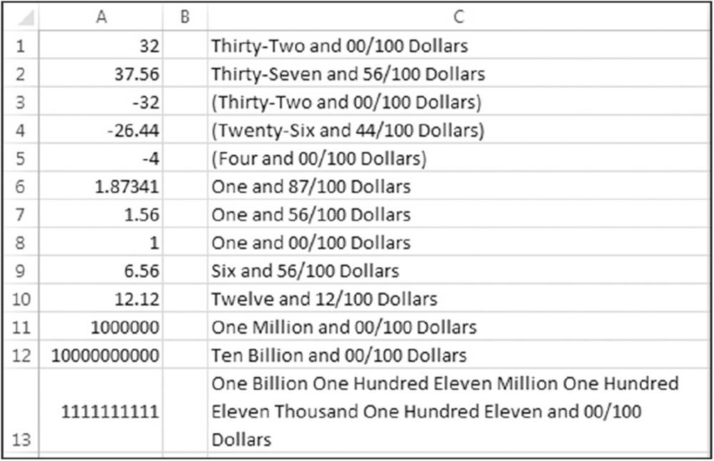
Figure 7.20 Examples of the SPELLDOLLARS function.
Note that negative numbers are spelled out and enclosed in parentheses.
On the Web
The SPELLDOLLARS function is too lengthy to list here, but you can view the complete listing in spelldollars function.xlsm on the book’s website.
A multifunctional function
The next example describes a technique that may be helpful in some situations: making a single worksheet function act like multiple functions. The following VBA listing is for a custom function called STATFUNCTION, which takes two arguments: the range (rng) and the operation (op). Depending on the value of op, the function returns a value computed using any of the following worksheet functions: AVERAGE, COUNT, MAX, MEDIAN, MIN, MODE, STDEV, SUM, or VAR.
For example, you can use this function in your worksheet as follows:
=STATFUNCTION(B1:B24,A24)
The result of the formula depends on the contents of cell A24, which should be a string such as Average, Count, or Max. You can adapt this technique for other types of functions.
Function STATFUNCTION (rng, op)
Select Case UCase(op)
Case"SUM"
STATFUNCTION = WorksheetFunction.Sum(rng)
Case"AVERAGE"
STATFUNCTION = WorksheetFunction.Average(rng)
Case"MEDIAN"
STATFUNCTION = WorksheetFunction.Median(rng)
Case"MODE"
STATFUNCTION = WorksheetFunction.Mode(rng)
Case"COUNT"
STATFUNCTION = WorksheetFunction.Count(rng)
Case"MAX"
STATFUNCTION = WorksheetFunction.Max(rng)
Case"MIN"
STATFUNCTION = WorksheetFunction.Min(rng)
Case"VAR"
STATFUNCTION = WorksheetFunction.Var(rng)
Case"STDEV"
STATFUNCTION = WorksheetFunction.StDev(rng)
Case Else
STATFUNCTION = CVErr(xlErrNA)
End Select
End Function
The SHEETOFFSET function
You probably know that Excel’s support for 3-D workbooks is limited. For example, if you need to refer to a different worksheet in a workbook, you must include the worksheet’s name in your formula. Adding the worksheet name isn’t a big problem . . . until you attempt to copy the formula across other worksheets. The copied formulas continue to refer to the original worksheet name, and the sheet references aren’t adjusted as they would be in a true 3-D workbook.
The example discussed in this section is the VBA SHEETOFFSET function, which enables you to address worksheets in a relative manner. For example, you can refer to cell A1 on the previous worksheet by using this formula:
=SHEETOFFSET(-1,A1)
The first argument represents the relative sheet, and it can be positive, negative, or zero. The second argument must be a reference to a single cell. You can copy this formula to other sheets, and the relative referencing will be in effect in all the copied formulas.
The VBA code for the SHEETOFFSET function follows:
Function SHEETOFFSET (Offset As Long, Optional Cell As Variant)
' Returns cell contents at Ref, in sheet offset
Dim WksIndex As Long, WksNum As Long
Dim wks As Worksheet
Application.Volatile
If IsMissing(Cell) Then Set Cell = Application.Caller
WksNum = 1
For Each wks In Application.Caller.Parent.Parent.Worksheets
If Application.Caller.Parent.Name = wks.Name Then
SHEETOFFSET = Worksheets(WksNum + Offset).Range(Cell(1).Address)
Exit Function
Else
WksNum = WksNum + 1
End If
Next wks
End Function
Returning the maximum value across all worksheets
If you need to determine the maximum value in cell B1 across a number of worksheets, you would use a formula such as this:
=MAX(Sheet1:Sheet4!B1)
This formula returns the maximum value in cell B1 for Sheet1, Sheet4, and all the sheets in between.
But what if you add a new sheet (Sheet5) after Sheet4? Your formula won’t adjust automatically, so you need to edit the formula to include the new sheet reference:
=MAX(Sheet1:Sheet5!B1)
The MaxAllSheets function accepts a single-cell argument and returns the maximum value in that cell across all worksheets in the workbook. The formula that follows, for example, returns the maximum value in cell B1 for all sheets in the workbook:
=MAXALLSHEETS(B1)
If you add a new sheet, you don’t need to edit the formula:
Function MAXALLSHEETS (cell)
Dim MaxVal As Double
Dim Addr As String
Dim Wksht As Object
Application.Volatile
Addr = cell.Range("A1").Address
MaxVal = -9.9E+307
For Each Wksht In cell.Parent.Parent.Worksheets
If Wksht.Name = cell.Parent.Name And _
Addr = Application.Caller.Address Then
' avoid circular reference
Else
If IsNumeric(Wksht.Range(Addr)) Then
If Wksht.Range(Addr) > MaxVal Then _
MaxVal = Wksht.Range(Addr).Value
End If
End If
Next Wksht
If MaxVal = -9.9E+307 Then MaxVal = 0
MAXALLSHEETS = MaxVal
End Function
The For Each statement uses the following expression to access the workbook:
cell.Parent.Parent.Worksheets
The parent of the cell is a worksheet, and the parent of the worksheet is the workbook. Therefore, the For Each-Next loop cycles among all worksheets in the workbook. The first If statement inside the loop performs a check to see whether the cell being checked is the cell that contains the function. If so, that cell is ignored to avoid a circular reference error.
Note
You can easily modify this function to perform other cross-worksheet calculations, such as minimum, average, and sum.
Returning an array of nonduplicated random integers
The function in this section, RANDOMINTEGERS, returns an array of nonduplicated integers. The function is intended to be used in a multicell array formula.
{=RANDOMINTEGERS()}
Select a range and then enter the formula by pressing Ctrl+Shift+Enter. The formula returns an array of nonduplicated integers, arranged randomly. For example, if you enter the formula into a 50-cell range, the formulas will return nonduplicated integers from 1 to 50.
The code for RANDOMINTEGERS follows:
Function RANDOMINTEGERS()
Dim FuncRange As Range
Dim V() As Variant, ValArray() As Variant
Dim CellCount As Double
Dim i As Integer, j As Integer
Dim r As Integer, c As Integer
Dim Temp1 As Variant, Temp2 As Variant
Dim RCount As Integer, CCount As Integer
' Create Range object
Set FuncRange = Application.Caller
' Return an error if FuncRange is too large
CellCount = FuncRange.Count
If CellCount > 1000 Then
RANDOMINTEGERS = CVErr(xlErrNA)
Exit Function
End If
' Assign variables
RCount = FuncRange.Rows.Count
CCount = FuncRange.Columns.Count
ReDim V(1 To RCount, 1 To CCount)
ReDim ValArray(1 To 2, 1 To CellCount)
' Fill array with random numbers
' and consecutive integers
For i = 1 To CellCount
ValArray(1, i) = Rnd
ValArray(2, i) = i
Next i
' Sort ValArray by the random number dimension
For i = 1 To CellCount
For j = i + 1 To CellCount
If ValArray(1, i) > ValArray(1, j) Then
Temp1 = ValArray(1, j)
Temp2 = ValArray(2, j)
ValArray(1, j) = ValArray(1, i)
ValArray(2, j) = ValArray(2, i)
ValArray(1, i) = Temp1
ValArray(2, i) = Temp2
End If
Next j
Next i
' Put the randomized values into the V array
i = 0
For r = 1 To RCount
For c = 1 To CCount
i = i + 1
V(r, c) = ValArray(2, i)
Next c
Next r
RANDOMINTEGERS = V
End Function
Randomizing a range
The RANGERANDOMIZE function, which follows, accepts a range argument and returns an array that consists of the input range — in random order:
Function RANGERANDOMIZE(rng)
Dim V() As Variant, ValArray() As Variant
Dim CellCount As Double
Dim i As Integer, j As Integer
Dim r As Integer, c As Integer
Dim Temp1 As Variant, Temp2 As Variant
Dim RCount As Integer, CCount As Integer
' Return an error if rng is too large
CellCount = rng.Count
If CellCount > 1000 Then
RANGERANDOMIZE = CVErr(xlErrNA)
Exit Function
End If
' Assign variables
RCount = rng.Rows.Count
CCount = rng.Columns.Count
ReDim V(1 To RCount, 1 To CCount)
ReDim ValArray(1 To 2, 1 To CellCount)
' Fill ValArray with random numbers
' and values from rng
For i = 1 To CellCount
ValArray(1, i) = Rnd
ValArray(2, i) = rng(i)
Next i
' Sort ValArray by the random number dimension
For i = 1 To CellCount
For j = i + 1 To CellCount
If ValArray(1, i) > ValArray(1, j) Then
Temp1 = ValArray(1, j)
Temp2 = ValArray(2, j)
ValArray(1, j) = ValArray(1, i)
ValArray(2, j) = ValArray(2, i)
ValArray(1, i) = Temp1
ValArray(2, i) = Temp2
End If
Next j
Next i
' Put the randomized values into the V array
i = 0
For r = 1 To RCount
For c = 1 To CCount
i = i + 1
V(r, c) = ValArray(2, i)
Next c
Next r
RANGERANDOMIZE = V
End Function
The code is similar to that for the RANDOMINTEGERS function. Remember to use this function as an array formula (by pressing Ctrl+Shift+Enter).
{=RANGERANDOMIZE(A2:A11)}
This formula returns the contents of A2:A11, but in a random order.
Sorting a range
The SORTED function accepts a single-column range argument and returns the range, sorted:
Function SORTED(Rng)
Dim SortedData() As Variant
Dim Cell As Range
Dim Temp As Variant, i As Long, j As Long
Dim NonEmpty As Long
' Transfer data to SortedData
For Each Cell In Rng
If Not IsEmpty(Cell) Then
NonEmpty = NonEmpty + 1
ReDim Preserve SortedData(1 To NonEmpty)
SortedData(NonEmpty) = Cell.Value
End If
Next Cell
' Sort the array
For i = 1 To NonEmpty
For j = i + 1 To NonEmpty
If SortedData(i) > SortedData(j) Then
Temp = SortedData(j)
SortedData(j) = SortedData(i)
SortedData(i) = Temp
End If
Next j
Next i
' Transpose the array and return it
SORTED = Application.Transpose(SortedData)
End Function
Enter the SORTED function as an array formula (by pressing Ctrl+Shift+Enter). The SORTED function returns the contents of a range, sorted.
The SORTED function starts by creating an array named SortedData. This array contains all nonblank values in the argument range. Next, the array is sorted, using a bubble sort algorithm. Because the array is a horizontal array, it must be transposed before it is returned by the function.
The SORTED function works with a range of any size, as long as it’s in a single column or row. If the unsorted data is in a row, your formula needs to use Excel’s TRANSPOSE function to display the sorted data horizontally. For example:
=TRANSPOSE(SORTED(A16:L16))
Windows API Calls
VBA has the capability to use functions that are stored in Dynamic Link Libraries (DLLs). DLLs expose functions and procedures used by the Windows operating system so that other programs can reach out and call these functions and procedures programmatically. This is referred to as making an application programming interface call (or an API call). The examples in this section illustrate the use of some common Windows API calls to DLLs.
Understanding API Declarations
When making Windows API calls, you’ll need to use an API declaration. An API declaration essentially tells Excel which Windows function or procedure you want to leverage, where it can be found, the parameters it takes, and what it returns.
For instance, the following API declaration calls the ability to play a sound file.
Public Declare Function PlayWavSound Lib"winmm.dll" _
Alias"sndPlaySoundA" (ByVal LpszSoundName As String, _
ByVal uFlags As Long) As Long
This tells Excel that:
· The function is Public (it can be used from any module).
· The function is going to be referred to in the code as PlayWavSound.
· The function is found in the winmm.dll file.
· It goes by the name of sndPlaySoundA in the DLL (this is case sensitive).
· It takes two parameters, a String that specifies the name of the sound file, and a Long number value that specifies any special method for playing the sound.
API declarations can be used just like any standard VBA function or procedure. The following example demonstrates how you would use the PlayWavSound API in a macro.
Public Declare PtrSafe Function PlayWavSound Lib"winmm.dll" Alias"sndPlaySoundA"_
(ByVal LpszSoundName As String, ByVal uFlags As Long) As LongPtr
Sub PlayChimes ()
PlayWavSound"C:\Windows\Media\Chimes.wav", 0
End Sub
32 Bit vs 64 Bit Declarations
With the introduction of 64 bit versions of Microsoft Office, many of the Windows API declarations had to be adjusted to account for the 64 bit platform. This means that a user with a 64 bit version of Excel installed will not be able to run code with older API declarations.
To avoid compatibility issues, you can use an extended declaration technique that ensures your API calls will work on both 32 bit and 64 bit Excel. Take a moment to review this example, which conditionally calls the ShellExecute API:
#If VBA7 Then
Private Declare PtrSafe Function ShellExecute Lib"shell32.dll" Alias _
"ShellExecuteA" (ByVal hwnd As LongPtr, ByVal lpOperation As String, _
ByVal lpFile As String, ByVal lpParameters As String, ByVal lpDirectory _
As String, ByVal nShowCmd As Long) As LongPtr
#Else
Private Declare Function ShellExecute Lib"shell32.dll" Alias"ShellExecuteA" _
(ByVal hwnd As Long, ByVal lpOperation As String, ByVal lpFile As _
String, ByVal lpParameters As String, ByVal lpDirectory As String, _
ByVal nShowCmd As Long) As Long
#End If
The pound sign (#) is used to mark conditional compilation. In this case, the first declaration will compile if the code is running on a 64bit version of Excel. If the code is running on a 32 bit version of Excel, the second declaration will compile.
Determining file associations
In Windows, many file types are associated with a particular application. This association makes it possible to double-click the file to load it into its associated application.
The following function, named GetExecutable, uses a Windows API call to get the full path to the application associated with a particular file. For example, your system has many files with a .txt extension — one named Readme.txt is probably in your Windows directory right now. You can use the GetExecutable function to determine the full path of the application that opens when the file is double-clicked.
Note
Windows API declarations must appear at the top of your VBA module.
Private Declare PtrSafe Function FindExecutableA Lib"shell32.dll" _
(ByVal lpFile As String, ByVal lpDirectory As String, _
ByVal lpResult As String) As Long
Function GetExecutable(strFile As String) As String
Dim strPath As String
Dim intLen As Integer
strPath = Space(255)
intLen = FindExecutableA(strFile,"\", strPath)
GetExecutable = Trim(strPath)
End Function
Figure 7.21 shows the result of calling the GetExecutable function, with an argument of the filename for an MP3 audio file. The function returns the full path of the application associated with the file.
Figure 7.21 Determining the path and name of the application associated with a particular file.
On the Web
This example is available on this book’s website in the file association.xlsm file.
Determining default printer information
The example in this section uses a Windows API function to return information about the active printer. The information is contained in a single text string. The example parses the string and displays the information in a more readable format.
Private Declare PtrSafe Function GetProfileStringA Lib"kernel32" _
(ByVal lpAppName As String, ByVal lpKeyName As String, _
ByVal lpDefault As String, ByVal lpReturnedString As _
String, ByVal nSize As Long) As Long
Sub DefaultPrinterInfo()
Dim strLPT As String * 255
Dim Result As String
Call GetProfileStringA _
("Windows","Device","", strLPT, 254)
Result = Application.Trim(strLPT)
ResultLength = Len(Result)
Comma1 = InStr(1, Result,",", 1)
Comma2 = InStr(Comma1 + 1, Result,",", 1)
' Gets printer's name
Printer = Left(Result, Comma1 - 1)
' Gets driver
Driver = Mid(Result, Comma1 + 1, Comma2 - Comma1 - 1)
' Gets last part of device line
Port = Right(Result, ResultLength - Comma2)
' Build message
Msg ="Printer:" & Chr(9) & Printer & Chr(13)
Msg = Msg &"Driver:" & Chr(9) & Driver & Chr(13)
Msg = Msg &"Port:" & Chr(9) & Port
' Display message
MsgBox Msg, vbInformation,"Default Printer Information"
End Sub
Note
The ActivePrinter property of the Application object returns the name of the active printer (and lets you change it), but there’s no direct way to determine what printer driver or port is being used. That’s why this function may be useful.
On the Web
This example is available on this book’s website in the printer info.xlsm file.
Determining video display information
The example in this section uses Windows API calls to determine a system’s current video mode for the primary display monitor. If your application needs to display a certain amount of information on one screen, knowing the display size helps you scale the text accordingly. In addition, the code determines the number of monitors. If more than one monitor is installed, the procedure reports the virtual screen size.
Declare PtrSafe Function GetSystemMetrics Lib"user32" _
(ByVal nIndex As Long) As Long
Public Const SM_CMONITORS = 80
Public Const SM_CXSCREEN = 0
Public Const SM_CYSCREEN = 1
Public Const SM_CXVIRTUALSCREEN = 78
Public Const SM_CYVIRTUALSCREEN = 79
Sub DisplayVideoInfo()
Dim numMonitors As Long
Dim vidWidth As Long, vidHeight As Long
Dim virtWidth As Long, virtHeight As Long
Dim Msg As String
numMonitors = GetSystemMetrics(SM_CMONITORS)
vidWidth = GetSystemMetrics(SM_CXSCREEN)
vidHeight = GetSystemMetrics(SM_CYSCREEN)
virtWidth = GetSystemMetrics(SM_CXVIRTUALSCREEN)
virtHeight = GetSystemMetrics(SM_CYVIRTUALSCREEN)
If numMonitors > 1 Then
Msg = numMonitors &" display monitors" & vbCrLf
Msg = Msg &"Virtual screen:" & virtWidth &" X"
Msg = Msg & virtHeight & vbCrLf & vbCrLf
Msg = Msg &"The video mode on the primary display is:"
Msg = Msg & vidWidth &" X" & vidHeight
Else
Msg = Msg &"The video display mode:"
Msg = Msg & vidWidth &" X" & vidHeight
End If
MsgBox Msg
End Sub
On the Web
This example is available on the book’s website in the video mode.xlsm file.
Reading from and writing to the Registry
Most Windows applications use the Windows Registry database to store settings. Your VBA procedures can read values from the Registry and write new values to the Registry. Doing so requires the following Windows API declarations:
Private Declare PtrSafe Function RegOpenKeyA Lib"ADVAPI32.DLL" _
(ByVal hKey As Long, ByVal sSubKey As String, _
ByRef hkeyResult As Long) As Long
Private Declare PtrSafe Function RegCloseKey Lib"ADVAPI32.DLL" _
(ByVal hKey As Long) As Long
Private Declare PtrSafe Function RegSetValueExA Lib"ADVAPI32.DLL" _
(ByVal hKey As Long, ByVal sValueName As String, _
ByVal dwReserved As Long, ByVal dwType As Long, _
ByVal sValue As String, ByVal dwSize As Long) As Long
Private Declare PtrSafe Function RegCreateKeyA Lib"ADVAPI32.DLL" _
(ByVal hKey As Long, ByVal sSubKey As String, _
ByRef hkeyResult As Long) As Long
Private Declare PtrSafe Function RegQueryValueExA Lib"ADVAPI32.DLL" _
(ByVal hKey As Long, ByVal sValueName As String, _
ByVal dwReserved As Long, ByRef lValueType As Long, _
ByVal sValue As String, ByRef lResultLen As Long) As Long
On the Web
On this book’s website, in a file named windows registry.xlsm, you will find two wrapper functions that greatly simplify the task of working with the Registry: GetRegistry and WriteRegistry. You will also find examples on how to put these wrapper functions to use.
Reading from the Registry
The GetRegistry function returns a setting from the specified location in the Registry. It takes three arguments:
· RootKey: A string that represents the branch of the Registry to address. This string can be one of the following:
· HKEY_CLASSES_ROOT
· HKEY_CURRENT_USER
· HKEY_LOCAL_MACHINE
· HKEY_USERS
· HKEY_CURRENT_CONFIG
· Path: The full path of the Registry category being addressed.
· RegEntry: The name of the setting to retrieve.
Here’s an example. If you’d like to find which graphic file, if any, is being used for the desktop wallpaper, you can call GetRegistry as follows. (Note that the arguments aren’t case-sensitive.)
RootKey ="hkey_current_user"
Path ="Control Panel\Desktop"
RegEntry ="Wallpaper"
MsgBox GetRegistry(RootKey, Path, RegEntry), _
vbInformation, Path &"\RegEntry"
The message box will display the path and filename of the graphic file (or an empty string if wallpaper isn’t used).
Writing to the Registry
The WriteRegistry function writes a value to the Registry at a specified location. If the operation is successful, the function returns True; otherwise, it returns False. WriteRegistry takes the following arguments (all of which are strings):
· RootKey: A string that represents the branch of the Registry to address. This string may be one of the following:
· HKEY_CLASSES_ROOT
· HKEY_CURRENT_USER
· HKEY_LOCAL_MACHINE
· HKEY_USERS
· HKEY_CURRENT_CONFIG
· Path: The full path in the Registry. If the path doesn’t exist, it is created.
· RegEntry: The name of the Registry category to which the value will be written. If it doesn’t exist, it is added.
· RegVal: The value that you’re writing.
Here’s an example that writes to the Registry a value representing the time and date Excel was started. The information is written in the area that stores Excel’s settings.
Sub Workbook_Open()
RootKey ="hkey_current_user"
Path ="software\microsoft\office\15.0\excel\LastStarted"
RegEntry ="DateTime"
RegVal = Now()
If WriteRegistry(RootKey, Path, RegEntry, RegVal) Then
msg = RegVal &" has been stored in the registry."
Else
msg ="An error occurred"
End If
MsgBox msg
End Sub
If you store this routine in the ThisWorkbook module in your Personal Macro Workbook, the setting is automatically updated whenever you start Excel.
An easier way to access the Registry
If you want to use the Windows Registry to store and retrieve settings for your Excel applications, you don’t have to bother with the Windows API calls. Rather, you can use the VBA GetSetting and SaveSetting functions. Using these functions is mucheasier than using the API calls.
These two functions are described in the Help system, so we won’t cover the details here. However, it’s important to understand that these functions work only with the following key name:
HKEY_CURRENT_USER\Software\VB and VBA Program Settings
In other words, you can’t use these functions to access any key in the registry. Rather, these functions are most useful for storing information about your Excel application that you need to maintain between sessions.
All materials on the site are licensed Creative Commons Attribution-Sharealike 3.0 Unported CC BY-SA 3.0 & GNU Free Documentation License (GFDL)
If you are the copyright holder of any material contained on our site and intend to remove it, please contact our site administrator for approval.
© 2016-2026 All site design rights belong to S.Y.A.