Marketing Analytics: Data-Driven Techniques with Microsoft Excel (2014)

Part III. Forecasting

Chapter 10. Using Multiple Regression to Forecast Sales

A common need in marketing analytics is forecasting the sales of a product. This chapter continues the discussion of causal forecasting as it pertains to this need. In causal forecasting, you try and predict a dependent variable (usually called Y) from one or more independent variables (usually referred to as X₁, X₂, …, X_n). In this chapter the dependent variable Y usually equals the sales of a product during a given time period.

Due to its simplicity, univariate regression (as discussed in Chapter 9, “Simple Linear Regression and Correlation”) may not explain all or even most of the variance in Y. Therefore, to gain better and more accurate insights about the often complex relationships between a variable of interest and its predictors, as well as to better forecast, one needs to move towards multiple regression in which more than one independent variable is used to forecast Y. Utilizing multiple regression may lead to improved forecasting accuracy along with a better understanding of the variables that actually cause Y.

For example, a multiple regression model can tell you how a price cut increases sales or how a reduction in advertising decreases sales. This chapter uses multiple regression in the following situations:

· Setting sales quotas for computer sales in Europe

· Predicting quarterly U.S. auto sales

· Understanding how predicting sales from price and advertising requires knowledge of nonlinearities and interaction

· Understanding how to test whether the assumptions needed for multiple regression are satisfied

· How multicollinearity and/or autocorrelation can disturb a regression model

Introducing Multiple Linear Regression

In a multiple linear regression model, you can try to predict a dependent variable Y from independent variables X₁, X₂, …X_n. The assumed model is as follows:

1

In Equation 1:

· B₀ is called the intercept or constant term.

· B_i is called the regression coefficient for the independent variable X_i.

The error term is a random variable that captures the fact that regression models typically do not fit the data perfectly; rather they approximate the relationships in the data. A positive value of the error term occurs if the actual value of the dependent variable exceeds your predicted value (B₀ +B₁X₁ + B₂X₂ + …B_nX_n). A negative value of the error term occurs when the actual value of the dependent variable is less than the predicted value.

The error term is required to satisfy the following assumptions:

· The error term is normally distributed.

· The variability or spread of the error term is assumed not to depend on the value of the dependent variable.

· For time series data successive values of the error term must be independent. This means, for example, that if for one observation the error term is a large positive number, then this tells you nothing about the value of successive error terms.

In the “Testing Validity of Multiple Regression Assumptions,” section of this chapter you will learn how to determine if the assumptions of regression analysis are satisfied, and what to do if the assumptions are not satisfied.

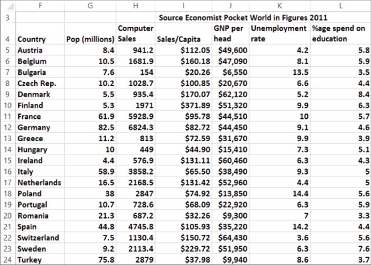
To best illustrate how to use multiple regression, the remainder of the chapter presents examples of its use based on a fictional computer sales company, HAL Computer. HAL sets sales quotas for all salespeople based on their territory. To set fair quotas, HAL needs a way to accurately forecast computer sales in each person's territory. From the 2011 Pocket World in Figures by The Economist, you can obtain the following data from 2007 (as shown in Figure 10.1 and file Europe.xlsx) for European countries:

· Population (in millions)

· Computer sales (in millions of U.S. dollars)

· Sales per capita (in U.S. dollars)

· GNP per head

· Average Unemployment Rate 2002–2007

· Percentage of GNP spent on education

Figure 10-1: HAL computer data

This data is cross-sectional data because the same dependent variable is measured in different locations at the same point in time. In time series data, the same dependent variable is measured at different times.

In order to apply the multiple linear regression model to the example, Y = Per Capital Computer spending, n = 3, X₁ = Per Capita GNP, X₂ = Unemployment Rate, and X₃ = Percentage of GNP spent on education.

Running a Regression with the Data Analysis Add-In

You can use the Excel Data Analysis Add-In to determine the best-fitting multiple linear regression equation to a given set of data. See Chapter 9 for a refresher on installation instructions for the Data Analysis Add-In.

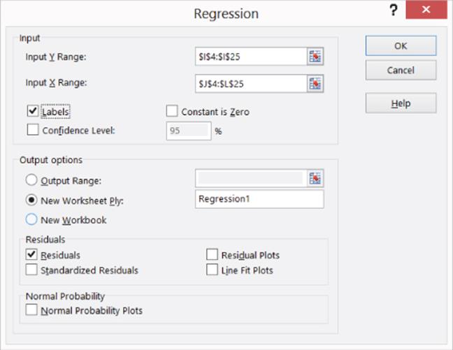
To run a regression, select Data Analysis in the Analysis Group on the Data tab, and then select Regression. When the Regression dialog box appears, fill it in, as shown in Figure 10.2.

· The Y Range (I4:I25) includes the data you want to predict (computer per capita sales), including the column label.

· The X Range (J4:L25) includes those values of the independent variables for each country, including the column label.

· Check the Labels box because your X range and Y range include labels. If you do not include labels in the X and Y range, then Excel will use generic labels like Y, X₁, X₂,…,X_n which are hard to interpret.

· The worksheet name Regression1 is the location where the output is placed.

· By checking the Residuals box, you can ensure Excel will generate the error (for each observation error = actual value of Y – predicted value for Y).

Figure 10-2: Regression dialog box

After selecting OK, Excel generates the output shown in Figures 10.3 and 10.4. For Figure 10.4, the highlighted text indicates data that is thrown out later in the chapter.

Figure 10-3: First multiple regression output

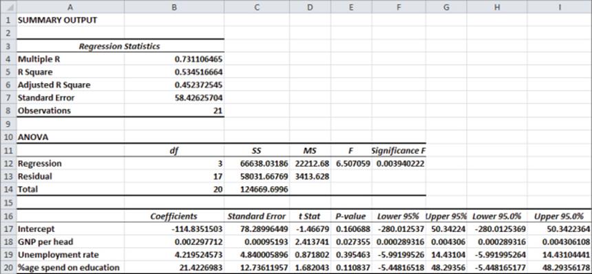
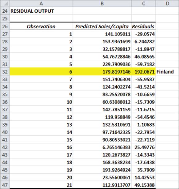
Figure 10-4: Residuals from first regression

Interpreting the Regression Output

After you run a regression, you next must interpret the output. To do this you must analyze a variety of elements listed in the output. Each element of the output affects the output in a unique manner. The following sections explain how to interpret the important elements of the regression output.

Coefficients

The Coefficients column of the output (cells B17:B20) gives the best fitting estimate of the multiple regression equation. Excel returns the following equation:

2

Excel found this equation by considering all values of B₀, B₁, B₂, and B₃ and choosing the values that minimize the sum over all observations of (Actual Dependent Variable – Predicted Value)². The coefficients are called the least squares estimates of B₀, B₁,…,B_n. You square the errors so positive and negative values do not cancel. Note that if the equation perfectly fits each observation, then the sum of squared errors is equal to 0.

F Test for Hypothesis of No Linear Regression

Just because you throw an independent variable into a regression does not mean it is a helpful predictor. If you used the number of games each country's national soccer team won during 2007 as an independent variable, it would probably be irrelevant and have no effect on computer sales. The ANOVA section of the regression output (shown in Figure 10.3) in cells A10:F14 enables you to test the following hypotheses:

· Null Hypothesis: The Hypothesis of No Linear Regression: Together all the independent variables are not useful (or significant) in predicting Y.

· Alternative Hypothesis: Together all the independent variables are useful (or significant).

To decide between these hypotheses, you must examine the Significance F Value in cell F12. The Significance F value of .004 tells you that the data indicates that there are only 4 chances in 1000 that your independent variables are not useful in predicting Y, so you would reject the null hypothesis. Most statisticians agree that a Significance F (often called p-value) of .05 or less should cause rejection of the Null Hypothesis.

Accuracy and Goodness of Fit of Regression Forecasts

After you conclude that the independent variables together are significant, a natural question is, how well does your regression equation fit the data? The R² value in B5 and Standard Error in B7 (see Figure 10.3) answer this question.

· The R² value of .53 indicates that 53 percent of the variation in Y is explained by Equation 1. Therefore, 47 percent of the variation in Y is unexplained by the multiple linear regression model.

· The Standard Error of 58.43 indicates that approximately 68 percent of the predictions for Y made from Equation 2 are accurate within one standard error ($58.43) and 95 percent of your predictions for Y made from Equation 2 are accurate within two standard errors ($116.86.)

Determining the Significant Independent Variables

Because you concluded that together your independent variables are useful in predicting Y, you now must determine which independent variables are useful. To do this look at the p-values in E17:E20. A p-value of .05 or less for an independent variable indicates that the independent variable is (after including the effects of all other independent variables in the equation) a significant predictor for Y. It appears that only GNP per head (p-value .027) is a significant predictor. At this point you want to see if there are any outliers or unusual data points. Outliers in regression are data points where the absolute value of the error (actual value of y – predicted value of y) exceeds two standard errors. Outliers can have a drastic effect on regression coefficients, and the analyst must decide whether to rerun the regression without the outliers.

The Residual Output and Outliers

For each data point or observation, the Residual portion of the regression output, as shown in Figure 10.4, gives you two pieces of information.

· The Predicted Value of Y from Equation 2. For example, Austria predicted per capita expenditures are given by the following:

· The Residuals section of the output gives for each observation the error = Actual value of Y – Predicted Value of Y. For Austria you find the residual is $112.05 – $141.10 = $–29.05. The regression equation found by least squares has the intuitively pleasing property that the sum of the residuals equals 0. This implies that overestimates and underestimates of Y cancel each other out.

Dealing with Insignificant Independent Variables

In the last section you learned that GNP per head was the only significant independent variable and the other two independent variables were insignificant. When an independent variable is insignificant (has a p-value greater than .05) you can usually drop it and run the regression again. Before doing this though, you must decide what to do with your outlier(s). Because the standard error or the regression is 58.4, any error exceeding 116.8 in absolute value is an outlier. Refer to Figure 10.4 and you can see that Finland (which is highlighted) is a huge outlier. Finland's spending on computers is more than three standard errors greater than expected. When you delete Finland as an outlier, and then rerun the analysis, the result is in the worksheet Regression2 of file Europe.xlsx, as shown in Figure 10.5.

Figure 10-5: Regression results: Finland outlier removed

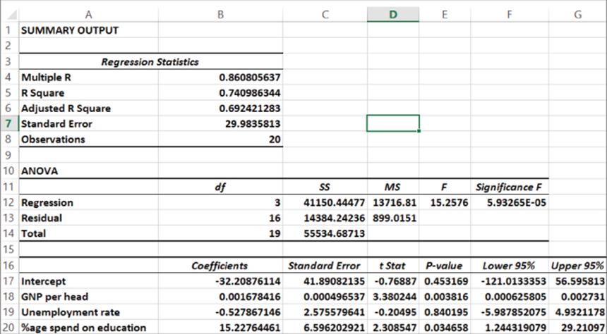
Checking the residuals you find that Switzerland is an outlier. (You under predict expenditures by slightly more than two standard errors.) Because Switzerland is not an outrageous outlier, you can choose to leave it in the data set in this instance. Unemployment Rate is insignificant (p-value of .84 > .05) so you can delete it from the model and run the regression again. The resulting regression is in worksheet Regression 3, of file Europe.xlsx as shown in Figure 10.6.

Figure 10-6: Regression output: unemployment rate removed

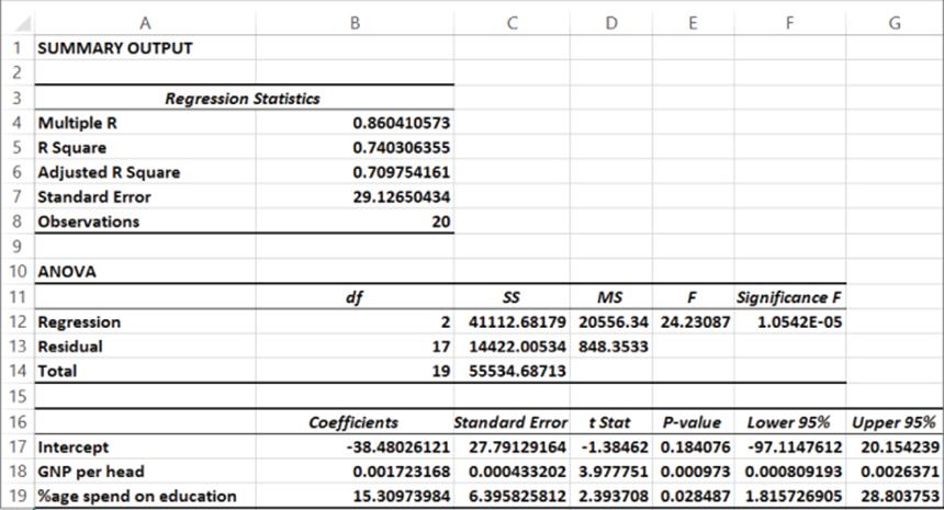
Both independent variables are significant, so use the following equation to predict Per Capita Computer Spending:

3

Because R² = 0.74, the equation explains 74 percent of the variation in Computer Spending. Because the Standard error is 29.13, you can expect 95 percent of your forecasts to be accurate within $58.26. From the Residuals portion of the output, you can see that Switzerland (error of $62.32) is the only outlier.

Interpreting Regression Coefficients

The regression coefficient of a variable estimates the effect (after adjusting for all other independent variables used to estimate the regression equation) of a unit increase in the independent variable. Therefore Equation 3 may be interpreted as follows:

· After adjusting for a fraction of GNP spent on education, a $1,000 increase in Per Capita GNP yields a $1.72 increase in Per Capital Computer spending.

· After adjusting for Per Capita GNP, a 1 percent increase in the fraction of GNP spent on education yields a $15.31 increase in Per Capita Computer spending.

Setting Sales Quotas

Often part of a salesperson's compensation is a commission based on whether a salesperson's sales quota is met. For commission payments to be fair, the company needs to ensure that a salesperson with a “good” territory has a higher quota than a salesperson with a “bad” territory. You'll now see how to use the multiple regression model to set fair sales quotas. Using the multiple regression, a reasonable annual sales quota for a territory equals the population * company market share * regression prediction for per capita spending.

Assume that a province in France has a per capita GNP of $50,000 and spends 10 percent of its GNP on education. If your company has a 30 percent market share, then a reasonable per capita annual quota for your sales force would be the following:

Therefore, a reasonable sales quota would be $60.23 per capita.

Beware of Blind Extrapolation

While you can use regressions to portray a lot of valuable information, you must be wary of using them to predict values of the independent variables that differ greatly from the values of the independent variables that fit the regression equation. For example, the Ivory Coast has a Per Capita GNP of $1,140, which is far less than any country in your European data set, so you could not expect Equation 3 to give a reasonable prediction for Per Capita Computer spending in the Ivory Coast.

Using Qualitative Independent Variables in Regression

In the previous example of multiple regression, you forecasted Per Capita Computer sales using Per Capita GNP and Fraction of GNP spent on education. Independent variables can also be quantified with an exact numerical value and are referred to as quantitative independent variables. In many situations, however, independent variables can't be easily quantified. This section looks at ways to incorporate a qualitative factor, such as seasonality, into a multiple regression analysis.

Suppose you want to predict quarterly U.S. auto sales to determine whether the quarter of the year impacts auto sales. Use the data in the file Autos.xlsx, as shown in Figure 10.7. Sales are listed in thousands of cars, and GNP is in billions of dollars.

Figure 10-7: Auto sales data

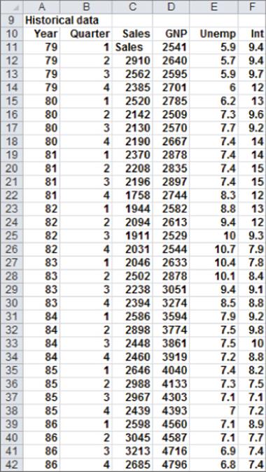
You might be tempted to define an independent variable that equals 1 during the first quarter, 2 during the second quarter, and so on. Unfortunately, this approach would force the fourth quarter to have four times the effect of the first quarter, which might not be true. The quarter of the year is a qualitative independent variable. To model a qualitative independent variable, create an independent variable (called a dummy variable) for all but one of the qualitative variable's possible values. (It is arbitrary which value you leave out. This example omits Quarter 4.) The dummy variables tell you which value of the qualitative variable occurs. Thus, you have a dummy variable for Quarter 1, Quarter 2, and Quarter 3 with the following properties:

· Quarter 1 dummy variable equals 1 if the quarter is Quarter 1 and 0 if otherwise.

· Quarter 2 dummy variable equals 1 if the quarter is Quarter 2 and 0 if otherwise.

· Quarter 3 dummy variable equals 1 if the quarter is Quarter 3 and 0 if otherwise.

A Quarter 4 observation can be identified because the dummy variables for Quarter 1 through Quarter 3 equal 0. It turns out you don't need a dummy variable for Quarter 4. In fact, if you include a dummy variable for Quarter 4 as an independent variable in your regression, Microsoft Office Excel returns an error message. The reason you get an error is because if an exact linear relationship exists between any set of independent variables, Excel must perform the mathematical equivalent of dividing by 0 (an impossibility) when running a multiple regression. In this situation, if you include a Quarter 4 dummy variable, every data point satisfies the following exact linear relationship:

(Quarter 1 Dummy)+(Quarter 2 Dummy)+(Quarter 3 Dummy)+(Quarter 4 Dummy)=1

NOTE

An exact linear relationship occurs if there exists constants c₀, c₁, … c_N, such that for each data point c₀ + c₁x₁ + c₂x₂ + … c_Nx_N = 0. Here x₁, … x_N are the values of the independent variables.

You can interpret the “omitted” dummy variable as a “baseline” scenario; this is reflected in the “regular” intercept. Therefore, you can think of dummies as changes in the intercept.

To create your dummy variable for Quarter 1, copy the formula IF(B12=1,1,0) from G12 to G13:G42. This formula places a 1 in column G whenever a quarter is the first quarter, and places a 0 in column G whenever the quarter is not the first quarter. In a similar fashion, you can create dummy variables for Quarter 2 (in H12:H42) and Quarter 3 (in I12:I42). Figure 10.8 shows the results of the formulas.

Figure 10-8: Dummy and lagged variables

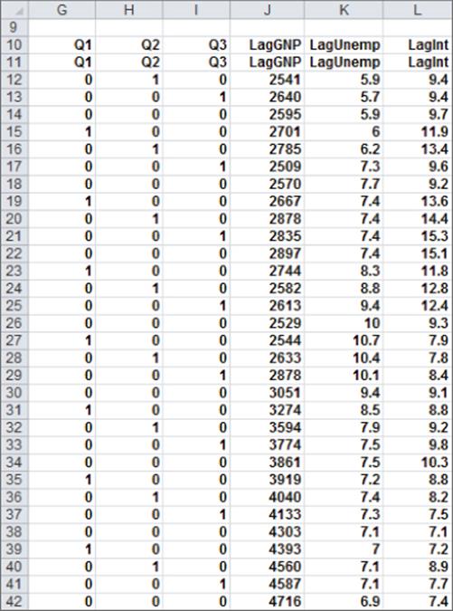
In addition to seasonality, you'd like to use macroeconomic variables such as gross national product (GNP, in billions of 1986 dollars), interest rates, and unemployment rates to predict car sales. Suppose, for example, that you want to estimate sales for the second quarter of 1979. Because values for GNP, interest rate, and unemployment rate aren't known at the beginning of the second quarter 1979, you can't use the second quarter 1979 GNP, interest rate, and unemployment rate to predict Quarter 2 1979 auto sales. Instead, you use the values for the GNP, interest rate, and unemployment rate lagged one quarter to forecast auto sales. By copying the formula =D11 from J12 to J12:L42, you can create the lagged value for GNP, the first of your macroeconomic-independent variables. For example, the range J12:L12 contains GNP, unemployment rate, and interest rate for the first quarter of 1979.

You can now run your multiple regression by clicking Data Analysis on the Data tab and then selecting Regression in the Data Analysis dialog box. Use C11:C42 as the Input Y Range and G11:L42 as the Input X Range; check the Labels box (row 11 contains labels), and also check the Residuals box. After clicking OK, you can obtain the output, which you can see in the Regression worksheet of the file Autos.xlsx and in Figure 10.9.

Figure 10-9: Summary regression output for auto example

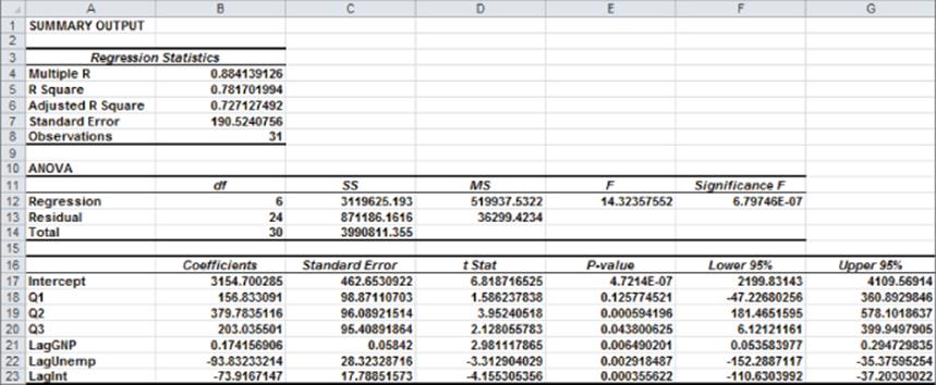
In Figure 10.9, you can see that Equation 1 is used to predict quarterly auto sales as follows:

Predicted quarterly sales=3154.7+156.833Q1+379.784Q2+203.03 6Q3+.174(LAGGNP in billions)–93.83(LAGUNEMP)–73.91(LAGINT)

Also in Figure 10.9, you see that each independent variable except Q1 has a p-value less than or equal to 0.05. The previous discussion would indicate that you should drop the Q1 variable and rerun the regression. Because Q2 and Q3 are significant, you know there is significant seasonality, so leave Q1 as an independent variable because this treats the seasonality indicator variables as a “package deal.” You can therefore conclude that all independent variables have a significant effect on quarterly auto sales. You interpret all coefficients in your regression equation ceteris paribus (which means that each coefficient gives the effect of the independent variable after adjusting for the effects of all other variables in the regression).

Each regression coefficient is interpreted as follows:

· A $1 billion increase in last quarter's GNP increases quarterly car sales by 174.

· An increase of 1 percent in last quarter's unemployment rate decreases quarterly car sales by 93,832.

· An increase of 1 percent in last quarter's interest rate decreases quarterly car sales by 73,917.

To interpret the coefficients of the dummy variables, you must realize that they tell you the effect of seasonality relative to the value left out of the qualitative variables. Therefore

· In Quarter 1, car sales exceed Quarter 4 car sales by 156,833.

· In Quarter 2, car sales exceed Quarter 4 car sales by 379,784.

· In Quarter 3, car sales exceed Quarter 4 car sales by 203,036.

Car sales are highest during the second quarter (April through June; tax refunds and summer are coming) and lowest during the third quarter. (October through December; why buy a new car when winter salting will ruin it?)

You should note that each regression coefficient is computed after adjusting for all other independent variables in the equation (this is often referred to as ceteris paribus, or all other things held equal).

From the Summary output shown in Figure 10.9, you can learn the following:

· The variation in your independent variables (macroeconomic factors and seasonality) explains 78 percent of the variation in your dependent variable (quarterly car sales).

· The standard error of your regression is 190,524 cars. You can expect approximately 68 percent of your forecasts to be accurate within 190,524 cars and about 95 percent of your forecasts to be accurate within 381,048 cars (2 * 190,524).

· There are 31 observations used to fit the regression.

The only quantity of interest in the ANOVA portion of Figure 10.9 is the significance (0.00000068). This measure implies that there are only 6.8 chances in 10,000,000, that when taken together, all your independent variables are useless in forecasting car sales. Thus, you can be quite sure that your independent variables are useful in predicting quarterly auto sales.

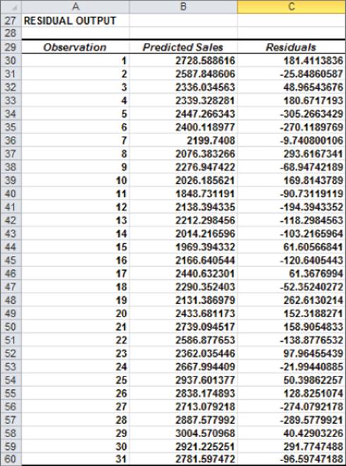
Figure 10.10 shows for each observation the predicted sales and residual. For example, for the second quarter of 1979 (observation 1), predicted sales from Equation 1 are 2728.6 thousand, and your residual is 181,400 cars (2910 – 2728.6). Note that no residual exceeds 381,000 in absolute value, so you have no outliers.

Figure 10-10: Residual output for Auto example

Modeling Interactions and Nonlinearities

Equation 1 assumes that each independent variable affects Y in a linear fashion. This means, for example, that a unit increase in X¹ will increase Y by B₁ for any values of X₁, X₂, …, X_n. In many marketing situations this assumption of linearity is unrealistic. In this section, you learn how to model situations in which an independent variable can interact with or influence Y in a nonlinear fashion.

Nonlinear Relationship

An independent variable can often influence a dependent variable through a nonlinear relationship. For example, if you try to predict product sales using an equation such as the following, price influences sales linearly.

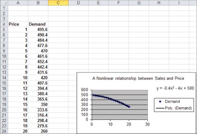
This equation indicates that a unit increase in price can (at any price level) reduce sales by 10 units. If the relationship between sales and price were governed by an equation such as the following, price and sales would be related nonlinearly.

As shown in Figure 10.11, larger increases in price result in larger decreases in demand. In short, if the change in the dependent variable caused by a unit change in the independent variable is not constant, there is a nonlinear relationship between the independent and dependent variables.

Figure 10-11: Nonlinear relationship between Sales and Price

Interaction

If the effect of one independent variable on a dependent variable depends on the value of another independent variable, you can say that the two independent variables exhibit interaction. For example, suppose you try to predict sales using the price and the amount spent on advertising. If the effect to change the level of advertising dollars is large when the price is low and small when the price is high, price and advertising exhibit interaction. If the effect to change the level of advertising dollars is the same for any price level, sales and price do not exhibit any interaction. You will encounter interactions again in Chapter 41, “Analysis of Variance: Two-way ANOVA.”

Testing for Nonlinearities and Interactions

To see whether an independent variable has a nonlinear effect on a dependent variable, simply add an independent variable to the regression that equals the square of the independent variable. If the squared term has a low p-value (less than 0.05), you have evidence of a nonlinear relationship.

To check whether two independent variables exhibit interaction, simply add a term to the regression that equals the product of the independent variables. If the term has a low p-value (less than 0.05), you have evidence of interaction. The file Priceandads.xlsx illustrates this procedure. In worksheet data from this file (see Figure 10.12), you have the weekly unit sales of a product, weekly price, and weekly ad expenditures (in thousands of dollars).

Figure 10-12: Nonlinearity and interaction data

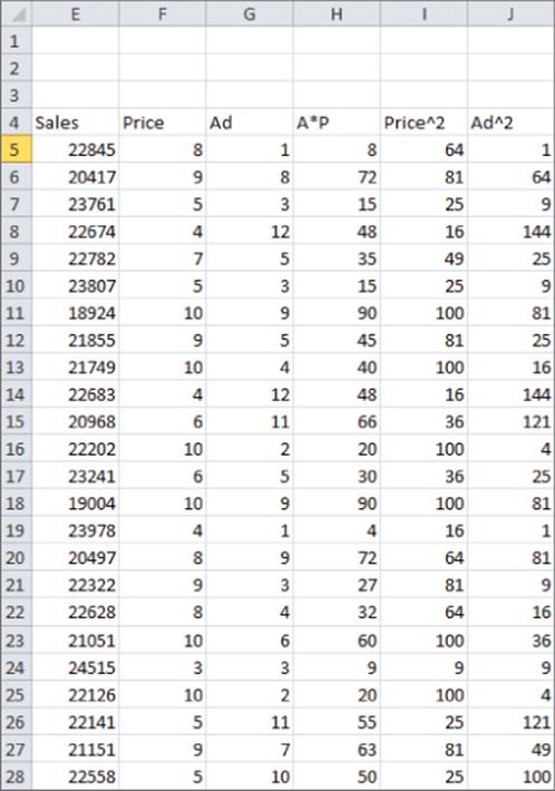
With this example, you'll want to predict weekly sales from the price and advertising. To determine whether the relationship is nonlinear or exhibits any interactions, perform the following steps:

1. Add in Column H Advertising*Price, in Column I Price², and in Column J Ad².

2. Next, run a regression with Y Range E4:E169 and X Range F4:J169. You can obtain the regression output, as shown in the worksheet nonlinear and Figure 10.13.

3. All independent variables except for Price² have significant p-values (less than .05). Therefore, drop Price² as an independent variable and rerun the regression. The result is in Figure 10.14 and the worksheet final.

Figure 10-13: First regression output for Nonlinearity and Interaction example

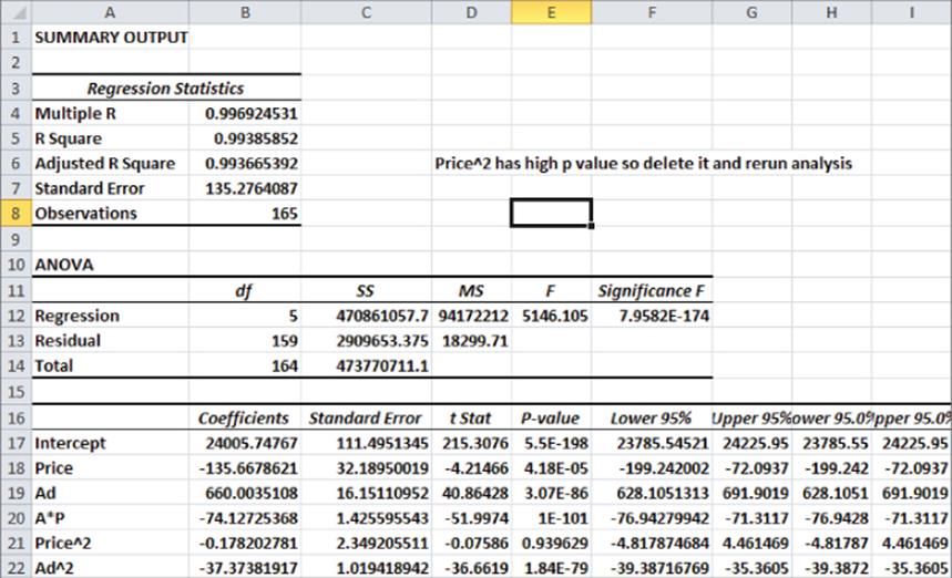
Figure 10-14: Final regression output for Nonlinearity and Interaction example

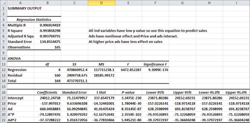
The Significance F Value is small, so the regression model has significant predictive values. All independent variables have extremely small p-values, so you can predict the weekly unit sales with the equation

The –37.33 Ad² term implies that each additional $1,000 in advertising can generate fewer sales (diminishing returns). The –74.13*Ad*P term implies that at higher prices additional advertising has a smaller effect on sales.

The R² value of 99.4 percent implies your model explains 99.4 percent of the variation in weekly sales. The Standard Error of 134.86 implies that roughly 95 percent of your forecasts should be accurate within 269.71. Interactions and non-linear effects are likely to cause multicollinearity, which is covered in the section “Multicollinearity” later in this chapter.

Testing Validity of Regression Assumptions

Recall earlier in the chapter you learned the regression assumptions that should be satisfied by the error term in a multiple linear regression. For ease of presentation, these assumptions are repeated here:

· The error term is normally distributed.

· The variability or spread of the error term is assumed not to depend on the value of the dependent variable.

· For time series data, successive values of the error term must be independent. This means, for example, that if for one observation the error term is a large positive number, then this tells you nothing about the value of successive error terms.

This section further discusses how to determine if these assumptions are satisfied, the consequences of violating the assumptions, and how to resolve violation of these assumptions.

Normally Distributed Error Term

You can infer the nature of an unknown error term through examination of the residuals. If the residuals come from a normal random variable, the normal random variable should have a symmetric density. Then the skewness (as measured by Excel SKEW function described in Chapter 2) should be near 0.

Kurtosis, which may sound like a disease but isn't, can also help you identify if the residuals are likely to have come from a normal random variable. Kurtosis near 0 means a data set exhibits “peakedness” close to the normal. Positive kurtosis means that a data set is more peaked than a normal random variable, whereas negative kurtosis means that data is less peaked than a normal random variable. The kurtosis of a data set may be computed with the Excel KURT function.

For different size data sets, Figure 10.15 gives 95 percent confidence intervals for the skewness and kurtosis of data drawn from a normal random variable.

Figure 10-15: 95 percent confidence interval for skewness and kurtosis for sample from a normal distribution

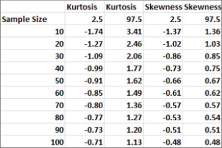
For example, it is 95 percent certain that in a sample of size 50 from a normal random variable, kurtosis is between –0.91 and 1.62. It is also 95 percent certain that in a sample of size 50 from a normal random variable, skewness is between –0.66 and 0.67. If your residuals yield a skewness or kurtosis outside the range shown in Figure 10.15, then you have reason to doubt the normality assumption.

In the computer spending example for European countries, you obtained a skewness of 0.83 and a kurtosis of 0.18. Both these numbers are inside the ranges specified in Figure 10.15, so you have no reason to doubt the normality of the residuals.

Non-normality of the residuals invalidates the p-values that you used to determine significance of independent variables or the entire regression. The most common solution to the problem of non-normal random variables is to transform the dependent variable. Often replacing y by Ln y, , or can resolve the non-normality of the errors.

Heteroscedasticity: A Nonconstant Variance Error Term

If larger values of an independent variable lead to a larger variance in the errors, you have violated the constant variance of the error term assumption, and heteroscedasticity is present. Heteroscedasticity, like non-normal residuals, invalidates the p-values used earlier in the chapter to test for significance. In most cases you can identify heteroscedasticity by graphing the predicted value on the x-axis and the absolute value of the residual on the y-axis. To see an illustration of this, look at the file Heteroscedasticity.xlsx. A sample of the data is shown in Figure 10.16.

Figure 10-16: Heteroscedasticity data

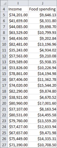
In this file, you are using the data in Heteroscedasticity.xlsx and trying to predict the amount a family spends annually on food from their annual income. After running a regression, you can graph the absolute value of the residuals against predicted food spending. Figure 10.17 shows the resulting graph.

Figure 10-17: Example of Heteroscedasticity

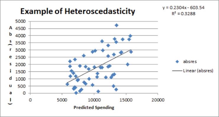
The upward slope of the line that best fits the graph indicates that your forecast accuracy decreases for families with more income, and heteroscedasticity is clearly present. Usually heteroscedasticity is resolved by replacing the dependent variable Y by Ln Y or . The reason why these transformations often resolve heteroscedasticity is that these transformations reduce the spread in the dependent variable. For example, if three data points have Y = 1, Y = 10,000 and Y = 1,000,000 then after using the transformation the three points now have a dependent variable with values 1, 100, and 1000 respectively.

Autocorrelation: The Nonindependence of Errors

Suppose your data is times series data. This implies the data is listed in chronological order. The auto data is a good example. The p-values used to test the hypothesis of no linear regression and the significance of an independent variable are not valid if your error terms appear to be dependent (nonindependent). Also, if your error terms are nonindependent, you can say that autocorrelation is present. If autocorrelation is present, you can no longer be sure that 95 percent of your forecasts will be accurate within two standard errors. Probably fewer than 95 percent of your forecasts will be accurate within two standard errors. This means that in the presence of autocorrelation, your forecasts can give a false sense of security. Because the residuals mirror the theoretical value of the error terms in Equation 1, the easiest way to see if autocorrelation is present is to look at a plot of residuals in chronological order. Recall the residuals sum to 0, so approximately half are positive and half are negative. If your residuals are independent, you would expect sequences of the form ++, + –, – +, and – – to be equally likely. Here + is a positive residual and – is a negative residual.

Graphical Interpretation of Autocorrelation

You can use a simple time series plot of residuals to determine if the error terms exhibit autocorrelation, and if so, the type of autocorrelation that is present.

Figure 10.18 shows an illustration of independent residuals exhibiting no autocorrelation.

Figure 10-18: Residuals indicate no autocorrelation

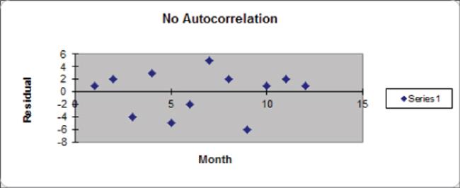
Here you can see 6 changes in sign out of 11 possible changes.

Figure 10.19, however, is indicative of positive autocorrelation. Figure 10.19 shows only one sign change out of 11 possible changes. Positive residuals are followed by positive residuals, and negative residuals are followed by negative residuals. Thus, successive residuals are positively correlated. When residuals exhibit few sign changes (relative to half the possible number of sign changes), positive autocorrelation is suspected. Unfortunately, positive autocorrelation is common in business and economic data.

Figure 10-19: Residuals indicate positive autocorrelation

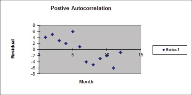
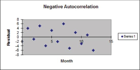
Figure 10.20 is indicative of negative autocorrelation. Figure 10.20 shows 11 sign changes out of a possible 11. This indicates that a small residual tends to be followed by a large residual, and a large residual tends to be followed a small residual. Thus, successive residuals are negatively correlated. This shows that many sign changes (relative to half the number of possible sign changes) are indicative of negative autocorrelation.

Figure 10-20: Residuals indicate negative autocorrelation

To help clarify these three different types of graphical interpretation, suppose you have n observations. If your residuals exhibit no correlation, then the chance of seeing either less than or more than sign changes is approximately 5 percent. Thus you can conclude the following:

· If you observe less than or equal to sign changes, conclude that positive autocorrelation is present.

· If you observe at least sign changes, conclude that negative autocorrelation is present.

· Otherwise you can conclude that no autocorrelation is present.

Detecting and Correcting for Autocorrelation

The simplest method to correct for autocorrelation is presented in the following steps. To simplify the presentation, assume there is only one independent variable (Call it X):

1. Determine the correlation between the following two time series: your residuals and your residuals lagged one period. Call this correlation p.

2. Run a regression with the dependent variable for time t being Y_t – pY_t-1 and independent variable X_t – pX_t-1.

3. Check the number of sign changes in the new regression's residuals. Usually, autocorrelation is no longer a problem, and you can rearrange your equation to predict Y_t from Y_t-1, X_t, and X_t-1.

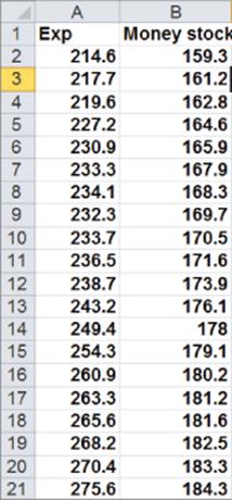
To illustrate this procedure, you can try and predict consumer spending (in billions of $) during a year as a function of the money supply (in billions of $). Twenty years of data are given in Figure 10.21 and are available for download from the file autocorr.xls.

Figure 10-21: Data for Autocorrelation example

Now complete the following steps:

1. Run a regression with X Range B1:B21 and Y Range A1:A21, and check the Labels and Residuals box. Figure 10.22 shows the residuals.

Figure 10-22: Residuals for Autocorrelation example

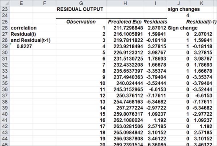
2. Observe that a sign change in the residuals occurs if, and only if, the product of two successive residuals is <0. Therefore, copying the formula =IF(I27*I26<0,1,0)from J27 to J28:J45 counts the number of sign changes. Compute the total number of sign changes (4) in cell J24 with the formula =SUM(J27:J45).

3. In cell J22 compute the “cutoff” for the number of sign changes that indicates the presence of positive autocorrelation. If the number of sign changes is <5.41, then you can suspect the positive autocorrelation is present: =9.5–SQRT(19).

4. Because you have only four sign changes, you can conclude that positive autocorrelation is present.

5. To correct for autocorrelation, find the correlation between the residuals and lagged residuals. Create the lagged residuals in K27:K45 by copying the formula =I26 from K27 to K28:K45.

6. Find the correlation between the residuals and lagged residuals (0.82) in cell L26 using the formula =CORREL(I27:I45, K27:K45).

7. To correct for autocorrelation run a regression with dependent variable Expenditures_t – .82 Expenditures_t–1 and independent variable Money Supply_t – .82 Money Supply_t–1. See Figure 10.23.

Figure 10-23: Transformed data to correct for autocorrelation

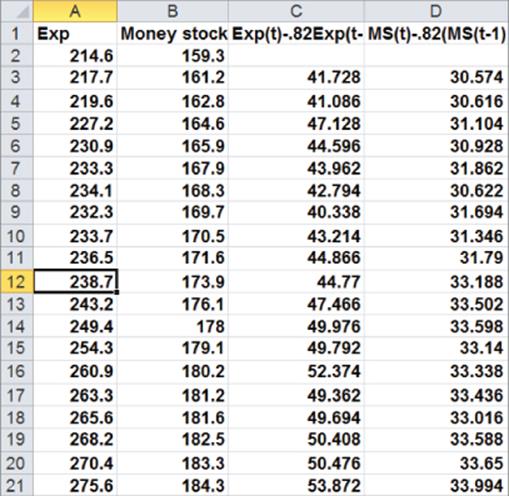
8. In Column C create your transformed dependent variable by copying the formula =A3-0.82*A2 from C3 to C4:C21.

9. Copy this same formula from D3 to D4:D21 to create the transformed independent variable Money Supply_t – .82Money Supply_t –₁.

10. Now run a regression with the Y Range as C3:C21 and X Range as D3:D21. Figure 10.24 shows the results.

Figure 10-24: Regression output for transformed data

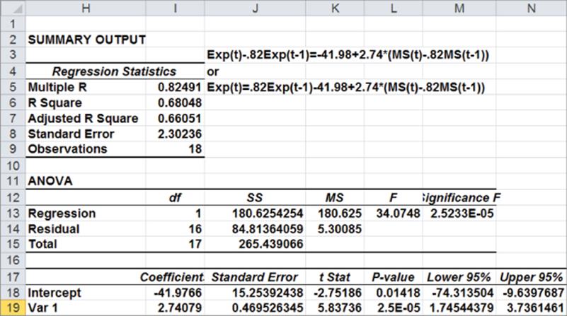
Because the p-value for your independent variable is less than .15, you can conclude that your transformed independent variable is useful for predicting your transformed independent variable. You can find the residuals from your new regression change sign seven times. This exceeds the positive autocorrelation cutoff of 4.37 sign changes. Therefore you can conclude that you have successfully removed the positive autocorrelation. You can predict period t expenditures with the following equation:

You can rewrite this equation as the following:

Because everything on the right hand side of the last equation is known at Period t, you can use this equation to predict Period t expenditures.

Multicollinearity

If two or more independent variables in a regression analysis are highly correlated, a regression analysis may yield strange results. Whenever two or more independent variables are highly correlated and the regression coefficients do not make sense, you can say that multicollinearity exists.

Figure 10.25 (see file housing.xls) gives the following data for the years 1963–1985: the number of housing starts (in thousands), U.S. population (in millions), and mortgage rate. You can use this data to develop an equation that can forecast housing starts by performing the following steps:

1. It seems logical that housing starts should increase over time, so include the year as an independent variable to account for an upward trend. The more people in the United States, the more housing starts you would expect, so include Housing Starts as an independent variable. Clearly, an increase in mortgage rates decreases housing starts, so include the mortgage rate as an independent variable.

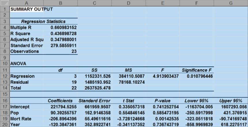
2. Now run a multiple regression with the Y range being A3:A26 and the X Range being B3:D26 to obtain the results shown in Figure 10.26.

3. Observe that neither POP nor YEAR is significant. (They have p-values of .59 and .74, respectively.) Also, the negative coefficient of YEAR indicates that there is a downward trend in housing starts. This doesn't make sense though. The problem is that POP and YEAR are highly correlated. To see this, use the DATA ANALYSIS TOOLS CORRELATION command to find the correlations between the independent variables.

4. Select Input Range B3:D26.

5. Check the labels box.

6. Put the output on the new sheet Correlation.

Figure 10-25: Multicollinearity data

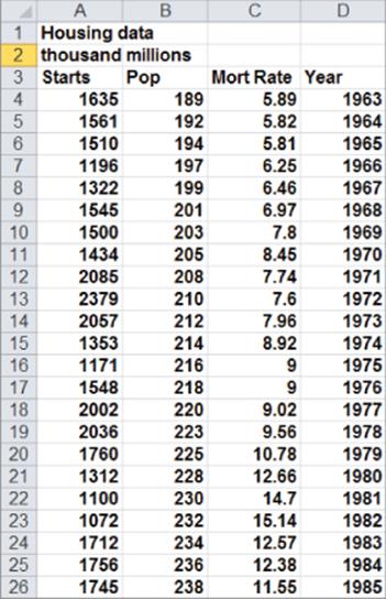
Figure 10-26: First regression output: Multicoillinearity example

You should obtain the output in Figure 10.27.

Figure 10-27: Correlation matrix for Multicollinearity example

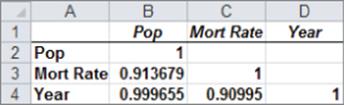
The .999 correlation between POP and YEAR occurs because both POP and YEAR increase linearly over time. Also note that the correlation between Mort Rate and the other two independent variables exceeds .9. Due to this, multicollinearity exists. What has happened is that the high correlation between the independent variables has confused the computer about which independent variables are important. The solution to this problem is to drop one or more of the highly correlated independent variables and hope that the independent variables remaining in the regression will be significant. If you decide to drop YEAR, change your X Range to B3:C26 to obtain the output shown in Figure 10.28. If you have access to a statistical package, such as SAS or SPSS, you can identify the presence of multicollinearity by looking at the Variance Inflation Factor (VIF) of each independent variable. A general rule of thumb is that any independent variable with a variance inflation factor exceeding 5 is evidence of multicollinearity.

Figure 10-28: Final regression output for Multicollinearity example

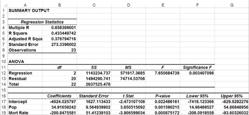
POP is now highly significant (p-value = .001). Also, by dropping YEAR you actually decreased s_e from 280 to 273. This decrease is because dropping YEAR reduced the confusion the computer had due to the strong correlation between POP and YEAR. The final predictive equation is as follows:

The interpretation of this equation is that after adjusting for interest rates, an increase in U.S. population of one million people results in $34,920 in housing starts. After adjusting for Population, an increase in interest rates of 1 percent can reduce housing starts by $200,850. This is valuable information that could be used to forecast the future cash flows of construction-related industries.

NOTE

After correcting for multicollinearity, the independent variables now have signs that agree with common sense. This is a common by-product of correcting for multicollinearity.

Validation of a Regression

The ultimate goal of regression analysis is for the estimated models to be used for accurate forecasting. When using a regression equation to make forecasts for the future, you must avoid over fitting a set of data. For example, if you had seven data points and only one independent variable, you could obtain an R² = 1 by fitting a sixth degree polynomial to the data. Unfortunately, such an equation would probably work poorly in fitting future data. Whenever you have a reasonable amount of data, you should hold back approximately 20 percent of your data (called the Validation Set) to validate your forecasts. To do this, simply fit regression to 80 percent of your data (called the Test Set). Compute the standard deviation of the errors for this data. Now use the equation generated from the Test Set to compute forecasts and the standard deviation of the errors for the Validation Set. Hopefully, the standard deviation for the Validation Set will be fairly close to the standard deviation for the Test Set. If this is the case, you can use the regression equation for future forecasts and be fairly confident that the accuracy of future forecasts will be approximated by the s_e for the Test Set. You can illustrate the important idea of validation with the data from your housing example.

Using the years 1963–1980 as your Test Set and the years 1981–1985 as the Validation Set, you can determine the suitability of the regression with independent variables POP and MORT RAT for future forecasting using the powerful TREND function. The syntax of the TREND function isTREND(known_y's,[known_x's],[new_x's],[const]). This function fits a multiple regression using the known y's and known x's and then uses this regression to make forecasts for the dependent variable using the new x's data. [Constant] is an optional argument. Setting [Constant]=False causes Excel to fit the regression with the constant term set equal to 0. Setting [Constant]=True or omitting [Constant] causes Excel to fit a regression in the normal fashion.

The TREND function is an array function (see Chapter 2) so you need to select the cell range populated by the TREND function and finally press Ctrl+Shift+Enter to enable TREND to calculate the desired results. As shown in Figure 10.29 and worksheet Data, you will now use the TREND function to compare the accuracy of regression predictions for the 1981-1985 validation period to the accuracy of regression predictions for the fitted data using the following steps.

1. To generate forecasts for the years 1963–1985 using the 1963–1980 data, simply select the range E4:E26 and enter in E4 the array formula =TREND(A4:A21, B4:C21,B4:C26) (refer to Figure 10.29). Rows 4-21 contain the data for the years 1963-1980 and Rows 4-26 contain the data for the years 1963-1985.

Figure 10-29: Use of Trend function to validate regression

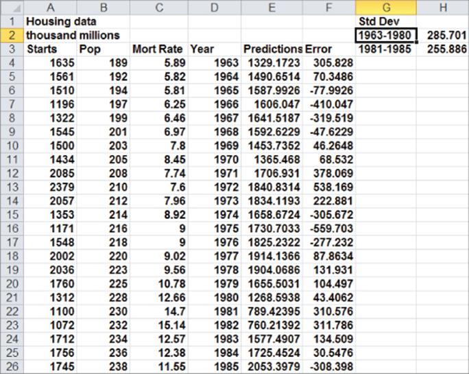
2. Compute the error for each year's forecast in Column F. The error for 1963 is computed in F4 with the formula =A4-F4.

3. Copy this formula down to row 26 to compute the errors for the years 1964–1985.

4. In cell H2 compute the standard deviation (285.70) of the errors for the years 1963–1980 with the formula =STDEV(F4:F21).

5. In cell H3 compute the standard deviation (255.89) of the forecast errors for the years 1981–1985 with the formula =AVERAGE(F22:F26).

The forecasts are actually more accurate for the Validation Set! This is unusual, but it gives you confidence that 95 percent of all future forecasts should be accurate within 2s_e = 546,700 housing starts.

Summary

In this chapter you learned the following:

· The multiple linear regression model models a dependent variable Y as B₀ + B₁X₁ + B₂X₂ +…B_nX_n + error term.

· The error term is required to satisfy the following assumptions:

· The error term is normally distributed.

· The variability or spread of the error term is assumed not to depend on the value of the dependent variable.

· For time series data, successive values of the error term must be independent. This means, for example, that if for one observation the error term is a large positive number, then this tells you nothing about the value of successive error terms.

· Violation of these assumptions can invalidate the p-values in the Excel output.

· You can run a regression analysis using the Data Analysis Tool.

· The Coefficients portion of the output gives the least squares estimates of B₀, B₁, …, B_n.

· A Significance F in the ANOVA section of the output less than .05 causes you to reject the hypothesis of no linear regression and conclude that your independent variables have significant predictive value.

· Independent variables with p-value greater than .05 should be deleted, and the regression should be rerun until all independent variables have p-values of .05 or less.

· Approximately 68 percent of predictions from a regression should be accurate within one standard error and approximately 95 percent of predictions from a regression should be accurate within two standard errors.

· Qualitative independent variables are modeled using indicator variables.

· By adding the square of an independent variable as a new independent variable, you can test whether the independent variable has a nonlinear effect on Y.

· By adding the product of two independent variables (say X₁ and X₂) as a new independent variable, you can test whether X₁ and X₂ interact in their effect on Y.

· You can check for the presence of autocorrelation in a regression based on time series data by examining the number of sign changes in the residuals; too few sign changes indicate positive autocorrelation and too many sign changes indicate negative autocorrelation.

· If independent variables are highly correlated, then their coefficients in a regression may be misleading. This is known as multicollinearity.

Exercises

1. Fizzy Drugs wants to optimize the yield from an important chemical process. The company thinks that the number of pounds produced each time the process runs depends on the size of the container used, the pressure, and the temperature. The scientists involved believe the effect to change one variable might depend on the values of other variables. The size of the process container must be between 1.3 and 1.5 cubic meters; pressure must be between 4 and 4.5 mm; and temperature must be between 22 and 30 degrees Celsius. The scientists patiently set up experiments at the lower and upper levels of the three control variables and obtain the data shown in the file Fizzy.xlsx.

(a) Determine the relationship between yield, size, temperature, and pressure.

(b) Discuss the interactions between pressure, size, and temperature.

(c) What settings for temperature, size, and pressure would you recommend?

2. For 12 straight weeks, you have observed the sales (in number of cases) of canned tomatoes at Mr. D's Supermarket. (See the file Grocery.xlsx.) Each week, you keep track of the following:

(a) Was a promotional notice for canned tomatoes placed in all shopping carts?

(b) Was a coupon for canned tomatoes given to each customer?

(c) Was a price reduction (none, 1, or 2 cents off ) given?

Use this data to determine how the preceding factors influence sales. Predict sales of canned tomatoes during a week in which you use a shopping cart notice, a coupon, and reduce price by 1 cent.

3. The file Countryregion.xlsx contains the following data for several underdeveloped countries:

· Infant mortality rate

· Adult literacy rate

· Percentage of students finishing primary school

· Per capita GNP

Use this data to develop an equation that can be used to predict infant mortality. Are there any outliers in this set of data? Interpret the coefficients in your equation. Within what value should 95 percent of your predictions for infant mortality be accurate?

4. The file Baseball96.xlsx gives runs scored, singles, doubles, triples, home runs, and bases stolen for each major league baseball team during the 1996 season. Use this data to determine the effects of singles, doubles, and other activities on run production.

5. The file Cardata.xlsx provides the following information for 392 different car models:

· Cylinders

· Displacement

· Horsepower

· Weight

· Acceleration

· Miles per gallon (MPG) Determine an equation that can predict MPG. Why do you think all the independent variables are not significant?

6. Determine for your regression predicting computer sales whether the residuals exhibit non-normality or heteroscedasticity.

7. The file Oreos.xlsx gives daily sales of Oreos at a supermarket and whether Oreos were placed 7” from the floor, 6” from the floor, or 5” from the floor. How does shelf position influence Oreo sales?

8. The file USmacrodata.xlsx contains U.S. quarterly GNP, Inflation rates, and Unemployment rates. Use this file to perform the following exercises:

(a) Develop a regression to predict quarterly GNP growth from the last four quarters of growth. Check for non-normality of residuals, heteroscedasticity, autocorrelation, and multicollinearity.

(b) Develop a regression to predict quarterly inflation rate from the last four quarters of inflation. Check for non-normality of residuals, heteroscedasticity, autocorrelation, and multicollinearity.

(c) Develop a regression to predict quarterly unemployment rate from the unemployment rates of the last four quarters. Check for non-normality of residuals, heteroscedasticity, autocorrelation, and multicollinearity.

9. Does our regression model for predicting auto sales exhibit autocorrelation, non-normality of errors, or heteroscedasticity?