Marketing Analytics: Data-Driven Techniques with Microsoft Excel (2014)

Part III. Forecasting

Chapter 13. Ratio to Moving Average Forecasting Method

In Chapter 12, “Modeling Trend and Seasonality,” you learned how to estimate trend and seasonal indices. Naturally you would like to use your knowledge of trend and seasonality to make accurate forecasts of future sales. The Ratio to Moving Average Method provides an accurate, easy-to-use forecasting method for future monthly or quarterly sales. This chapter shows how to use this method to easily estimate seasonal indices and forecast future sales.

Using the Ratio to Moving Average Method

The simple Ratio to Moving Average Forecasting Method is described in this section via examples using data from the Ratioma.xlsx file, which includes sales of a product during 20 quarters (as shown in Figure 13.1 in rows 5 through 24). This technique enables you to perform two tasks:

· Easily estimate a time series' trend and seasonal indices.

· Generate forecasts of future values of the time series.

Figure 13-1: Example of Ratio to Moving Average Method

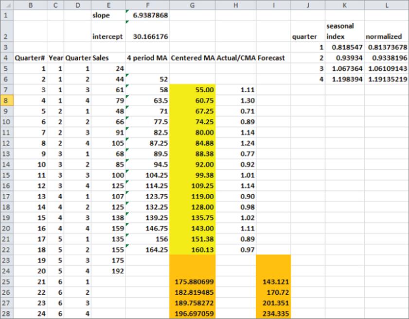
Using the first 20 quarters for the data exemplified in this chapter, you will be able to forecast sales for the following four quarters (Quarters 21 through 24). Similar to the one in Chapter 12, this time series data has both trend and seasonality.

The Ratio to Moving Average Method has four main steps:

· Estimate the deseasonalized level of the series during each period (using centered moving averages).

· Fit a trend line to your deseasonalized estimates (in Column G).

· Determine the seasonal index for each quarter and estimate the future level of the series by extrapolating the trend line.

· Predict future sales by reseasonalizing the trend line estimate.

The following sections walk you through each main part of this process.

Calculating Moving Averages and Centered Moving Averages

To begin, you compute a four-quarter (four quarters eliminates seasonality) moving average for each quarter by averaging the prior quarter, current quarter, and next two quarters. To do this you copy the formula =AVERAGE(E5:E8) down from cell F6 to F7:F22. For example, for Quarter 2, the moving average is (24 + 44 + 61 + 79) / 4 = 52.

Because the moving average for Quarter 2 averages Quarters 1 through 4 and the numbers 1–4 average to 2.5, the moving average for Quarter 2 is centered at Quarter 2.5. Similarly, the moving average for Quarter 3 is centered at Quarter 3.5. Therefore, averaging these two moving averages gives a centered moving average that estimates the level of the process at the end of Quarter 3. To estimate the level of the series during each series (without seasonality), copy the formula =AVERAGE(F6:F7) down from cell G7.

Fitting a Trend Line to the Centered Moving Averages

You can use the centered moving averages to fit a trend line that can be used to estimate the future level of the series. To do so, follow these steps:

1. In cell F1 use the formula =SLOPE(G7:G22,B7:B22) to find the slope of the trend line.

2. In cell F2 use the formula =INTERCEPT(G7:G22,B7:B22) to find the intercept of the trend line.

3. Estimate the level of the series during Quarter t to be 6.94t c + 30.17.

4. Copy the formula =intercept + slope*B25 down from cell G25 to G26:G28 to compute the estimated level (excluding seasonality) of the series from Quarter 21 onward.

Compute the Seasonal Indexes

Recall that a seasonal index of 2 for a quarter means sales in that quarter are twice the sales during an average quarter, whereas a seasonal index of .5 for a quarter would mean that sales during that quarter were one-half of an average quarter. Therefore, to determine the seasonal indices, begin by determining for each quarter for which you have sales (Actual Sales) / Centered Moving Average. To do this, copy the formula =E7/G7 down from cell H7 to H8:H22. You find, for example, that during Quarter 1 sales were 77 percent, 71 percent, 90 percent and 89 percent of average, so you could estimate the seasonal index for Quarter 1 as the average of these four numbers (82 percent). To calculate the initial seasonal index estimates, you can copy the formula =AVERAGEIF($D$7:$D$22,J3,$H$7:$H$22) from cell K3 to K4:K6. This formula averages the four estimates you have for Q1 seasonality.

Unfortunately, the seasonal indices do not average exactly to 1. To ensure that your final seasonal indices average to 1, copy the formula =K3/AVERAGE($K$3:$K$6) from cell L3 to L4:L6.

Forecasting Sales during Quarters 21–24

To create your sales forecast for each future quarter, simply multiply the trend line estimate for the quarter's level (from Column G) by the appropriate seasonal index. Copy the formula =VLOOKUP(D25,season,3)*G25 from cell G25 to G26:G28 to compute the final forecast for Quarters 21–24. This forecast includes estimates of trend and seasonality.

If you think the trend of the series has changed recently, you can estimate the series' trend based on more recent data. For example, you could use the centered moving averages for Quarters 13–18 to get a more recent trend estimate by using the formula =SLOPE(G17:G22,B17:B22). This yields an estimated trend of 8.09 units per quarter. If you want to forecast Quarter 22 sales, for example, you take the last centered moving average you have (from Quarter 18) of 160.13 and add 4 (8.09) to estimate the level of the series in Quarter 22. Then multiply the estimate of the Quarter 22 level by the Quarter 2 seasonal index of .933 to yield a final forecast for Quarter 22 sales of (160.13 + 4(8.09)) * (.933) = 179.6 units.

Applying the Ratio to Moving Average Method to Monthly Data

Often the Ratio to Moving Average Method is used to forecast monthly sales as well as quarterly sales. To illustrate the application of this method to monthly data, let's look at U.S. housing starts.

The Housingstarts.xlsx file gives monthly U.S. housing starts (in thousands) for the period January 2000 through May 2011. Based on the data through November 2010, you can apply the Ratio to Moving Average Method to forecast monthly U.S. housing starts for the period December 2010 through May 2011. You can forecast a total of 3.5 million housing starts, and in reality there were 3.374 million housing starts. The key difference between applying the method to monthly and quarterly data is that for monthly data you need to use 12-month moving averages to eliminate seasonality.

Summary

In this chapter you learned the following:

· Applying the Ratio to Moving Average Method involves the following tasks:

· Compute four-quarter moving averages and then determine the centered moving averages.

· Fit a trend line to the centered moving averages.

· Compute seasonal indices.

· Compute forecasts for future periods.

· You can apply the Ratio to Moving Average Method to monthly data as well by following the same process but use 12-month moving averages to eliminate seasonality.

Exercises

1. The file Walmartdata.xls contains quarterly revenues of Wal-Mart during the years 1994–2009. Use the Ratio to Moving Average Method to forecast revenues for Quarters 3 and 4 in 2009 and Quarters 1 and 2 in 2010. Use Quarters 53–60 to create a trend estimate that you use in your forecasts.

2. Based on the data in the file airlinemiles.xlsx from Chapter 12, use the Ratio to Moving Average Method to forecast airline miles for the remaining months in 2012.