Marketing Analytics: Data-Driven Techniques with Microsoft Excel (2014)
Part III. Forecasting
Chapter 14. Winter's Method
Predicting future values of a time series is usually difficult because the characteristics of any time series are constantly changing. For instance, as you saw in Chapter 12, “Modeling Trend and Seasonality,” the trend in U.S. airline passenger miles changed several times during the 2000–2012 period.Smoothing or adaptive methods are usually best suited for forecasting future values of a time series. Essentially, smoothing methods create forecasts by combining information from a current observation with your prior view of a parameter, such as trend or a seasonal index. Unlike many other smoothing methods, Winter's Method incorporates both trend and seasonal factors. This makes it useful in situations where trend and seasonality are important. Because in an actual situation (think U.S. monthly housing starts) trend and seasonality are constantly changing, a method such as Winter's Method that changes trend and seasonal index estimates during each period has a better chance of keeping up with changes than methods like the trend and seasonality approaches based on curve fitting discussed in Chapter 12, which use constant estimates of trend and seasonal indices.
To help you understand how Winter's Method works, this chapter uses it to forecast airline passenger miles for April through December 2012 based on the data studied in Chapter 12. This chapter describes the three key characteristics of a time series (level, trend, and seasonality) and explains the initialization process, notation, and key formulas needed to implement Winter's Method. Finally, you explore forecasting with Winter's Method and the concept of Mean Absolute Percentage Error (MAPE).
Parameter Definitions for Winter's Method
In this chapter you will develop Winter's exponential smoothing method using the three time series characteristics, level (also called base), trend, and seasonal index, discussed in Chapter 12 in the “Multiplicative Model with Trend and Seasonality” section. After observing data through the end of month t you can estimate the following quantities of interest:
· Lt = Level of series
· Tt = Trend of series
· St = Seasonal index for current month
The key to Winter's Method is the use of the following three equations, which are used to update Lt, Tt, and St. In the following equations, alp, bet, and gam are called smoothing parameters. The values of these parameters will be chosen to optimize your forecasts. In the following equations, cequals the number of periods in a seasonal cycle (c = 12 months for example) and xt equals the observed value of the time series at time t.
1 ![]()
2 ![]()
3 ![]()
Equation 1 indicates that the new base estimate is a weighted average of the current observation (deseasonalized) and last period's base is updated by the last trend estimate. Equation 2 indicates that the new trend estimate is a weighted average of the ratio of the current base to last period's base (this is a current estimate of trend) and last period's trend. Equation 3 indicates that you update the seasonal index estimate as a weighted average of the estimate of the seasonal index based on the current period and the previous estimate. In equations 1–3 the first term uses an estimate of the desired quantity based on the current observation and the second term uses a past estimate of the desired quantity.
NOTE
Note that larger values of the smoothing parameters correspond to putting more weight on the current observation.
You can define Ft,k as your forecast (F) after period t for the period t + k. This results in the following equation:
4 ![]()
Equation 4 first uses the current trend estimate to update the base k periods forward. Then the resulting base estimate for period t + k is adjusted by the appropriate seasonal index.
Initializing Winter's Method
To start Winter's Method, you must have initial estimates for the series base, trend, and seasonal indices. You can use the data from the airline winters.xls file, which contains monthly U.S. airline passenger miles for the years 2003 and 2004 to obtain initial estimates of level, trend, and seasonality. See Figure 14.1.
Figure 14-1: Data for Winter's Method
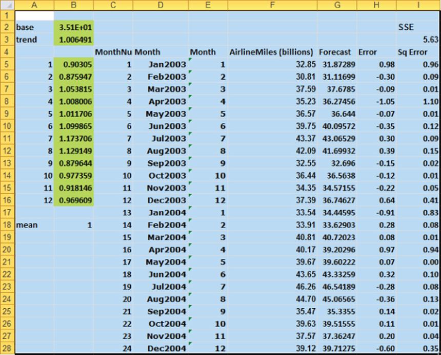
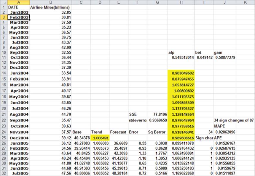
In the Initial worksheet you can fit the Multiplicative Trend Model from Chapter 12 to the 2003–2004 data. As shown in Figure 14.2, you use the trend and seasonal index from this fit as the original seasonal index and the December 2004 trend. Cell C25 determines an estimate of the base for December 2004 by deseasonalizing the observed December 2004 miles. This is accomplished with the formula =(B25/H25).
Figure 14-2: Initialization of Winter's Method
The next part of Winter's Method includes choosing the smoothing parameters to optimize the one-month-ahead forecasts for the years 2005 through 2012.
Estimating the Smoothing Constants
After observing each month's airline miles (in billions), you are now ready to update the smoothing constants. In Column C, you will update the series base; in Column D, the series trend; and in Column H, the seasonal indices. In Column E, you compute the forecast for next month, and in Column G, you compute the squared error for each month. Finally, you'll use Solver to choose smoothing constant values that minimize the sum of the squared errors. To enact this process, perform the following steps:
1. In H11:J11, enter trial values (between 0 and 1) for the smoothing constants.
2. In C26:C113, compute the updated series level with Equation 1 by copying the formula =alp*(B26/H14)+(1–alp)*(C25*D25) from cell C26 to C27:C113.
3. In D26:D113, use Equation 2 to update the series trend. Copy the formula =bet*(C26/C25)+(1-bet)*D25 cell from D26 to D27:D113.
4. In H26:H113, use Equation 3 to update the seasonal indices. Copy the formula =gam*(B26/C26)+(1-gam)*H14 from cell H26 to H27:H113.
5. In E26:E113, use Equation 4 to compute the forecast for the current month by copying the formula =(C25*D25)*H14 from cell E26 to E27:E113.
6. In F26:F113 compute each month's error by copying the formula =(B26-E26) from cell E26 to E27:E113.
7. In G26:G113, compute the squared error for each month by copying the formula =F26^2 from cell F26 to F27:F113. In cell G21 compute the Sum of Squared Errors (SSE) using the formula =SUM(G26:G113).
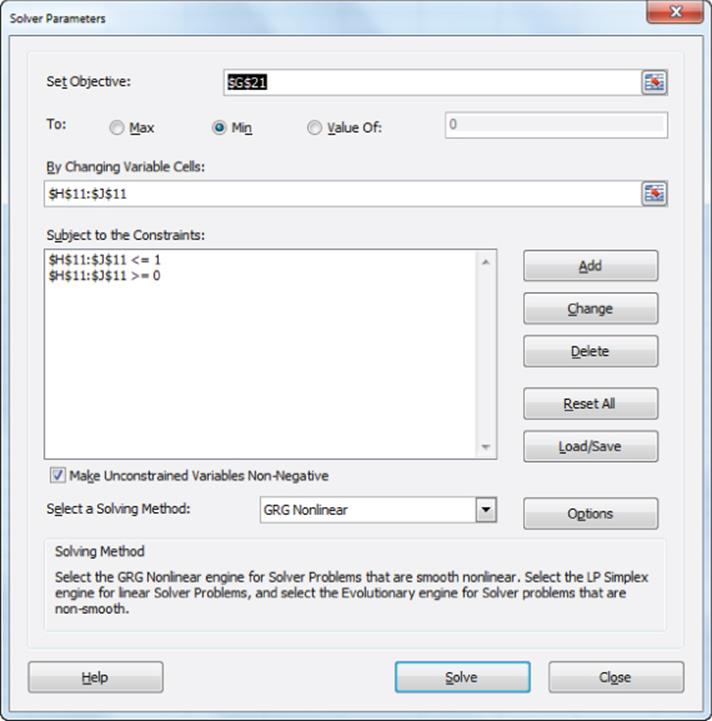
8. Now use the Solver to determine smoothing parameter values that minimize SSE. The Solver Parameters dialog box is shown in Figure 14.3.
9. Choose the smoothing parameters (H11:J11) to minimize SSE (cell G21). The Excel Solver ensures you can find the best combination of smoothing constants. Smoothing constants must be α The Solver finds that alp = 0.55, bet = 0.05, and gamma = 0.59.
Figure 14-3: Solver Window for optimizing smoothing constants
Forecasting Future Months
Now that you have estimated the Winter's Method smoothing constants α, β, γ, etc.), you are ready to use these estimates to forecast future airline miles. This can be accomplished using the formula in cell D116. Copying this formula down to cells D117:D123 enables you to forecast sales for the months of May through December of 2012. Figure 14.4 offers a visual summary of the forecasted sales.
Figure 14-4: Forecasting with Winter's Method
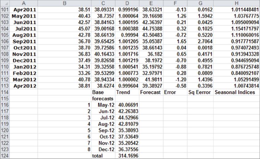
Figure 14.4 shows the forecasted sales for May through December 2012 by copying the formula =($C$113*$D$113^B116)*H102 from cell D116 to D117:D123. Cell D124 adds up these forecasts and predicts the rest of 2012 to see 314.17 billion airline miles traveled.
Cell G22 computes the standard deviation (0.94 billion) of the one-month-ahead forecast errors. This implies that approximately 95 percent of the forecast errors should be at most 1.88 billion. From Column F you see none of the one-month-ahead forecasts are outliers.
Mean Absolute Percentage Error (MAPE)
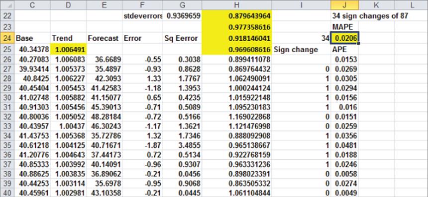
Statisticians like to estimate parameters for a forecast model by minimizing squared errors. In reality, however, most people are more interested in measuring forecast accuracy by looking at the Mean of Absolute Percentage Error (MAPE). This is probably because MAPE, unlike SSE, is measured in the same units as the data. Figure 14.5 shows that the one-month-ahead forecasts are off by an average of 2.1 percent. To compute the Absolute Percentage Error (APE) for each month, copy the formula =ABS(B26-E26)/B26 from cell G26 to J26:J113. In cell J24 the formula =AVERAGE(J26:J113)computes the MAPE.
Figure 14-5: Computation of MAPE
Winter's Method is an attractive forecasting method for several reasons:
· Given past data, the method can easily be programmed to provide quick forecasts for thousands of products.
· Winter's Method catches changes in trend or seasonality.
· Smoothing methods “adapt” to the data. That is, if you underforecast you raise parameter estimates and if you overforecast you lower parameter estimates.
Summary
In this chapter you learned the following:
· Exponential smoothing methods update time series parameters by computing a weighted average of the estimate of the parameter from the current observation with the prior estimate of the parameter.
· Winter's Method is an exponential smoothing method that updates the base, trend, and seasonal indices after each equation:
(1) Lt = alp(xt) / (st–c) + (1–alp)(Lt–1 * Tt–1 )
(2) Tt = bet(Lt / Lt–1) + (1–bet)Tt–1
(3) St = gam(xt / Lt) + (1–gam)s(t–c)
· Forecasts for k periods ahead at the end of period t are made with Winter's Method using Equation 4:
(4) Ft,k = Lt * (Tt)kst+k–c
Exercises
All the data for the following exercises can be found in the file Quarterly.xlsx.
1. Use Winter's Method to forecast one-quarter-ahead revenues for Wal-Mart.
2. Use Winter's Method to forecast one-quarter-ahead revenues for Coca-Cola.
3. Use Winter's Method to forecast one-quarter-ahead revenues for Home Depot.
4. Use Winter's Method to forecast one-quarter-ahead revenues for Apple.
5. Use Winter's Method to forecast one-quarter-ahead revenues for Amazon.com.
6. Suppose at the end of 2007 you were predicting housing starts in Los Angeles for the years 2008 and 2009. Why do you think Winter's Method would provide better forecasts than multiple regression?
All materials on the site are licensed Creative Commons Attribution-Sharealike 3.0 Unported CC BY-SA 3.0 & GNU Free Documentation License (GFDL)
If you are the copyright holder of any material contained on our site and intend to remove it, please contact our site administrator for approval.
© 2016-2026 All site design rights belong to S.Y.A.