Marketing Analytics: Data-Driven Techniques with Microsoft Excel (2014)

Part IV. What do Customers Want?

Chapter 16: Conjoint Analysis

Chapter 17: Logistic Regression

Chapter 18: Discrete Choice Analysis

Chapter 16. Conjoint Analysis

Often the marketing analyst is asked to determine the attributes of a product that are most (and least) important in driving a consumer's product choice. For example, when a soda drinker chooses between Coke and Pepsi, what is the relevant importance of the following:

· Price

· Brand (Coke or Pepsi)

· Type of soda (diet or regular)

After showing a consumer several products (called product profiles) and asking the consumer to rank these product profiles, the analyst can use full profile conjoint analysis to determine the relative importance of various attributes. This chapter shows how the basic ideas behind conjoint analysis are simply an application of multiple regression as explained in Chapter 10, “Using Multiple Regression to Forecast Sales.”

After understanding how to estimate a conjoint model, you will learn to use conjoint analysis to develop a market simulator, which can determine how a product's market share can change if the product's attributes are changed or if a new product is introduced into the market.

The chapter closes with a brief discussion of two other forms of conjoint analysis: adaptive/hybrid conjoint and choice-based conjoint.

Products, Attributes, and Levels

Essentially, conjoint analysis enables the marketing analyst to determine the product characteristics that drive a consumer's preference for products. For example, in purchasing a new car what matters most: brand, price, fuel efficiency, styling, or engine power? Conjoint analysis analyzes the consumer decision process by identifying the number of product choices available; listing the main characteristics used by consumers when choosing among products; and ranking each attribute offered in each product. After learning a few definitions, you will work through a detailed illustration of conjoint analysis.

The product set is a set of objects from which the consumer must make a choice (choosing no product is often an option). For example, a product set might be luxury sedans, laptop computers, shampoos, sodas, and so on. Conjoint analysis is also used in fields such as human resources, so product sets don't necessarily have to be consumer goods. For example, the HR analyst might want to determine what type of compensation mix (salary, bonus, stock options, vacation days, and telecommuting) is most attractive to prospective hires.

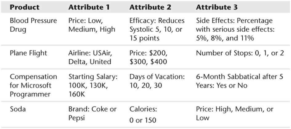
Each product is defined by the level of several product attributes. Attributes are the variables that describe the product. The levels for each attribute are the possible values of the attributes. Table 16.1 shows four examples of levels and attributes.

Table 16.1 Examples of Product Attributes and Levels

The purpose of conjoint analysis is to help the marketing analyst understand the relative importance of the attributes and within each attribute the ranking of the levels. For example, a customer might rank the attributes in order of importance for price, brand, and food service. The customer might rank the brands in the order of Marriott, Hilton, and Holiday Inn. The best-known application of conjoint analysis is its use to design the Courtyard Marriott Hotel chain. This study is described in Wind, Green, Shifflet, and Scarborough's journal article, “Courtyard by Marriott: Designing a Hotel Facility with Consumer-Based Marketing Models” (Interfaces, 1989, pp. 25–47). This study used the following product attributes:

· External décor

· Room décor

· Food service

· Lounge facilities

· General services

· Leisure facilities

· Security features

Other industries in which conjoint analysis has been used to ascertain how consumers value various product attributes include comparisons of the following:

· Credit card offers

· Health insurance plans

· Automobiles

· Overnight mail services (UPS versus FedEx)

· Cable TV offerings

· Gasoline (Shell versus Texaco)

· Ulcer drugs

· Blood pressure drugs

· E-ZPass automated toll paying versus toll booths

The best way to learn how to use conjoint analysis is to see it in action. The following section works through a complete example that shows how conjoint analysis can give you knowledge of customer preferences.

Full Profile Conjoint Analysis

To illustrate the use of full profile conjoint analysis, this section uses a classic example that is described in Paul Green and Yorman Wind's article “New Way to Measure Consumers' Judgments” (Harvard Business Review, August 1975, pp. 107–17, http://hbr.org/1975/07/new-way-to-measure-consumers-judgments/ar/1). The goal of this conjoint study was to determine the role that five attributes play in influencing a consumer's preference for carpet cleaner. The five attributes (and their levels) deemed relevant to the consumer preference are as follows:

· Package design (either A, B, or C)

· Brand (1, 2, or 3)

· Price (either $1.19, $1.39, or $1.59)

· Did Good Housekeeping magazine approve product?

· Is product guaranteed?

These attributes were chosen not just because they are measurable, but because the researchers believed these attributes were likely to drive consumer product choices.

Determining the Product Profiles

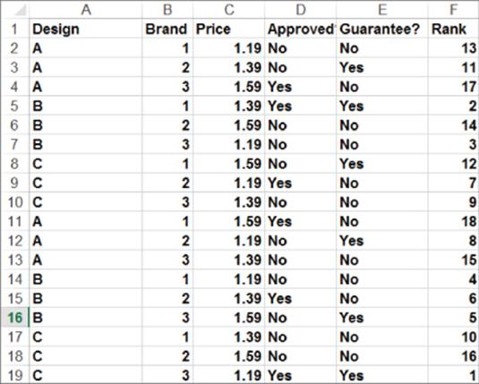
In full profile conjoint analysis, the consumer is shown a set of products (called product profiles) and asked to rank them in order from best (#1) to worst. In the carpet cleaning situation there are a total of 3 × 3 × 3 × 2 × 2 = 108 possible product profiles. It seems unlikely that any consumer could rank the order of 108 product combinations; therefore, the marketing analyst must show the consumer a much smaller number of combinations. Green and Wind chose to show the consumer the 18 possible combinations shown in Figure 16.1. After being shown these combinations, the consumer ranked the product profiles (refer to Figure 16.1). Here a rank of 1 indicates the most preferred product profile and a rank of 18 the least preferred product profile. For example, the consumer felt the most preferred product was Package C, Brand 3, $1.19 price, with a guarantee and Good Housekeeping Seal. This data is available in the Data worksheet of the conjoint.xls file that is available for download from the companion website.

Figure 16-1: Data for conjoint example

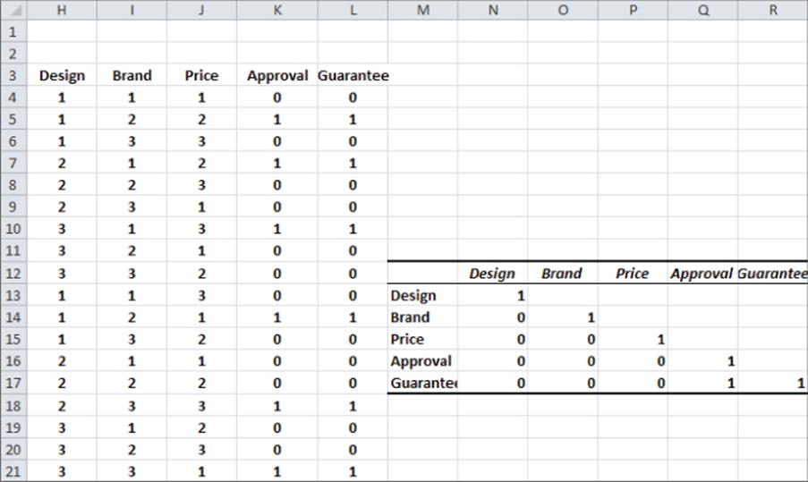
The 18 product profiles cannot be randomly chosen. For example, if every profile with a guarantee also had Good Housekeeping approval, then the analyst could not determine whether the consumer preferred a profile due to a guarantee or a Good Housekeeping approval. Essentially, you want the attributes to be uncorrelated, so with few product profiles, a multiple regression will be less likely to be “confused” by the correlation between attributes. Such a combination of product profiles is called an orthogonal design. Figure 16.2 shows that the product profiles from Figure 16.1 yield an orthogonal design.

Figure 16-2: Proof design is orthogonal.

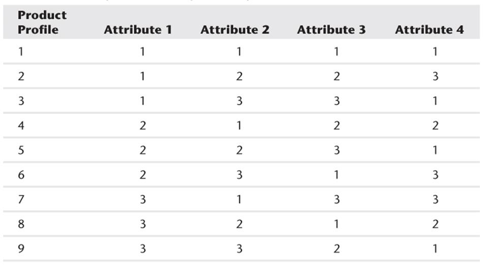
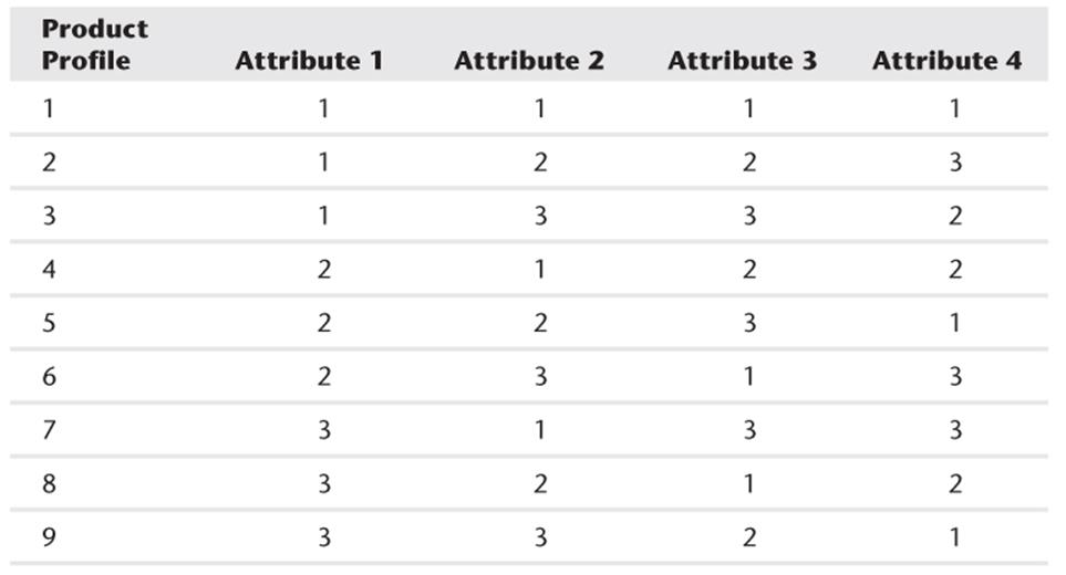
Sidney Adelman's article “Orthogonal Main-Effect Plans for Asymmetrical Factorial Experiments” (Technometric, 1962, Vol. 4 No. 1, pp. 36–39) is an excellent source on orthogonal designs. Table 16.2 illustrates an orthogonal design with nine product profiles and four attributes, each having three levels. For example, the first product profile sets each attribute to level 1.

Table 16.2 Example of an Orthogonal Design

Running the Regression

You can determine the relative importance of product attributes by using regression with dummy variables. You begin by rescaling the consumer's rankings so that the highest ranked product combination receives a score of 18 and the lowest ranked product combination receives a score of 1. This ensures that the larger regression coefficients for product attributes correspond to more preferred attributes. Without the rescaling, the larger regression coefficients would correspond to less preferred attributes. The analysis applies the following steps to the information in the Data worksheet:

1. Rescale the product profile rankings by subtracting 19 from the product combination's actual ranking. This yields the rescaled rankings called the inverse rankings.

2. Run a multiple linear regression using dummy variables to determine the effect of each product attribute on the inverse rankings.

3. This requires leaving out an arbitrarily chosen level of each attribute; for this example you can leave out Design C, Brand 3, a $1.59 price, no Good Housekeeping Seal, and no guarantee.

After rescaling the rankings a positive coefficient for a dummy variable indicates that the given level of the attribute makes the product more preferred than the omitted level of the attribute, and a negative coefficient for a dummy variable indicates that the given level of the attribute makes the product less preferred than the omitted level of the attribute. Figure 16.3 displays the coding of the data.

Figure 16-3: Coding of conjoint data

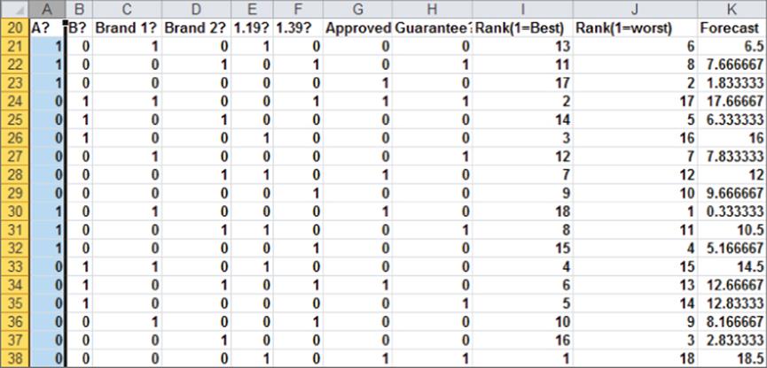
Notice how Row 21 indicates that if you charge $1.19 for Brand 1 and Package design A with no guarantee or Good Housekeeping approval, the combination is rated 6th from worst (or 13th overall). If you run a regression with Y-range J21:J38 and X-range A21:H38, you can obtain the equation shown in Figure 16.4 (see the Regression worksheet).

Figure 16-4: Conjoint regression data

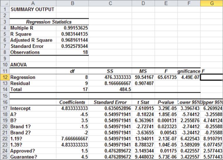
All independent variables are significant at the .05 level. (All p-values are smaller than .05.) The R² value of 0.98 indicates that the attributes explain 98 percent of the variation in this consumer's ranking. As discussed in Chapter 10, “Using Multiple Regression to Forecast Sales,” the standard error of 0.95 indicates that 95 percent of the predicted ranks would be accurate within 1.9. Thus it appears that the multiple linear regression model adequately captures how this consumer processes a product and creates a product ranking.

If the multiple linear regression model for a conjoint analysis does not produce a high R² and a low standard error, it is likely that one of the following must have occurred:

· You omitted some attributes that the consumer feels are important.

· The consumer's preferences are related to the current set of attributes via an interaction and nonlinear relationship. You can test for interactions or nonlinear relationships using the techniques described in Chapter 10.

The best prediction for the rescaled rank of a product is as follows:

1

To interpret this equation, recall from the discussion of dummy variables in Chapter 11 that all coefficients are interpreted relative to the level of the attribute that was coded with all 0s. This observation implies the following:

· Design C leads to a rank 4.5 higher than Design A and 3.5 lower than Design B.

· Brand 3 leads to a rank 1.5 higher than Brand 1 and 2 higher than Brand 2.

· A $1.19 price leads to a rank 7.67 higher than $1.59 and 2.83 higher than $1.39.

· A Good Housekeeping approval yields a rank 1.5 better than no approval.

· A guarantee yields a rank 4.5 higher than no guarantee.

By array entering the formula =TREND(J21:J38,A21:H38,A21:H38) in the range K21:K38, you create the predicted inverse rank for each product profile. The close agreement between Columns J and K shows how well a simple multiple linear regression explains this consumer's product profile rankings.

Ranking the Attributes and Levels

Which attributes have the most influence on the customer's likelihood to purchase the product? To rank the importance of the attributes, order the attributes based on the attributes' spread from the best level of the attribute to the worst level of the attribute. Table 16.3 displays this ranking.

Table 16.3 Product Attribute Rankings

For example, you can see the package design is the most important attribute and the Good Housekeeping approval is the least important attribute. You can also rank the levels within each attribute. This customer ranks levels as follows:

· Design: B, C, A

· Price: $1.19, $1.39, $1.59

· Brand: Brand 3, Brand 1, Brand 2

· Guarantee: Guarantee, No Guarantee

· Approval: Approval, No Approval

Within each attribute, you can rank the levels from most preferred to least preferred. In this customer's example, Brand 3 is most preferred, Brand 1 is second most preferred, and Brand 2 is least preferred.

Using Conjoint Analysis to Segment the Market

You can also use conjoint analysis to segment the market. To do so, simply determine the regression equation described previously for 100 representative customers. Let each row of your spreadsheet be the weights each customer gives to each attribute in the regression. Thus for the customer analyzed in the preceding section, his row would be (–4.5, 3.5, -1.5, –2, 7.67, 4.83, 1.5, 4.5). Then perform a cluster analysis (see Chapter 23, “Cluster Analysis”) to segment customers. This customer, for example, would be representative of a brand-insensitive, price-elastic decision maker who thought package design was critical.

Value-Based Pricing with Conjoint Analysis

Many companies price their products using cost plus pricing. For example, a cereal manufacturer may mark up the cost of producing a box of cereal by 20 percent when selling to the retailer. Cost plus pricing is prevalent for several reasons:

· It is simple to implement, even if your company sells many different products.

· Product margins are maintained at past levels, thereby reducing shareholder criticism that “margins are eroding.”

· Price increases can be justified if costs increase.

Unfortunately, cost plus pricing ignores the voice of the customer. Conjoint analysis, on the other hand, can be used to determine the price that can be charged for a product feature based on the value consumers attach to that feature. For example, how much is a Pentium 4 worth versus a Pentium 2? How much can a hotel charge for high-speed wireless Internet access? The key idea is that Equation 1 enables you to impute a monetary value for each level of a product attribute. To illustrate how conjoint analysis can aid in value-based pricing, assume the preferences of all customers in the carpet cleaning example are captured by Equation 1. Suppose the carpet cleaning fluid without guarantee currently sells for $1.39. What can you charge if you add a guarantee? You can implement value-based pricing by keeping the product with a guarantee at the same value as a product without a guarantee at the current price of $1.39.

The regression implies the following:

· $1.19 has a score of 7.67.

· $1.39 has a score of 4.83.

· $1.59 has a score of 0.

Thus, increasing the product price (in the range $1.39 to $1.59) by 1 cent costs you 4.83/20 = 0.24 points.

Because a guarantee increases ranking by 4.5 points, value-based pricing says that with a guarantee you should increase price by x cents where 0.24x = 4.5 or x = 4.5/0.24 = 19 cents.

You should check that if the product price is increased by 19 cents (to $1.58) and the product is guaranteed, the customer will be as happy as she was before. This shows that you have priced the guarantee according to the customer's imputed value. Although this approach to value-based pricing is widely used, it does not ensure profit maximization. When you study discrete choice in Chapter 18, “Discrete Choice Analysis,” you will see how choice-based conjoint analysis can be used to incorporate consumer preferences into profit maximization. Of course, this analysis assumes that for a price between $1.39 and $1.59 the effect of price on product ranking is a linear function of price. If this is not the case then Price² should have been added to the regression as an independent variable. This would allow the regression to capture the nonlinear effect of price on the consumer's product rankings.

Using Evolutionary Solver to Generate Product Profiles

The leading statistical packages (SAS and SPSS) enable a user to input a desired number of product profiles, the number of attributes, and the number of levels, and output (if one exists) an orthogonal design. In many situations the user must exclude product profiles that are unreasonable. For example, in analyzing an automobile it is unreasonable to set the car's size to a Mini Cooper and assume the car can carry six passengers. This section shows how to use the Excel 2010 or 2013 Evolutionary Solver to easily design something that is close to being orthogonal but that excludes unreasonable product profiles. The work here is based on Steckel, DeSarbo, and Mahajan's study “On the Creation of Acceptable Conjoint Analysis Experimental Designs” (Decision Sciences, 1991, pp. 436–42, http://goo.gl/2PO0J) and can be found in the evconjoint.xlsx file. If desired, the reader may omit this advanced section without loss of continuity.

Assume that you want to use a conjoint analysis to evaluate how consumers value the following attributes for a new car:

· Miles per gallon (MPG): 20 or 40

· Maximum speed in miles per hour (MPH): 100 or 150

· Length: 12 feet or 14 feet

· Price: $25,000 or $40,000

· Passenger capacity: 4, 5, or 6

Now suppose the analyst wants to create 12 product profiles and exclude the following types of product profiles as infeasible:

· 40 MPG, 6 passengers, 14-foot car

· 14-foot car, 150 MPH, and $20,000 price

· 40 MPG and 150 MPH

You can now see how to design 12 product profiles that include each level of an attribute an equal number of times, which are close to orthogonal and exclude infeasible product profiles.

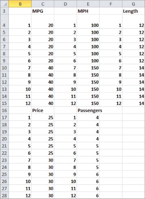
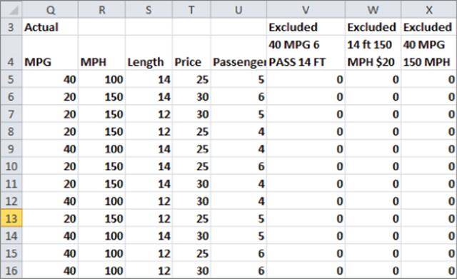
1. To begin, list in B3:G28 each attribute and level the number of times you want the combination to occur in the profiles. For example, Figure 16.5 lists 20 MPG six times and four passengers four times.

Figure 16-5: Listing attribute-level combinations

2. Give a range name to each listing of attribute values. For the example file the range D16:E28 is named lookpassengers.

3. The key to the model is to determine in cells K5:O16 how to “scramble” (as shown in Figure 16.6) for each attribute the integers 1 through 12 to select for each product profile the level for each attribute.

Figure 16-6: Selecting attribute levels

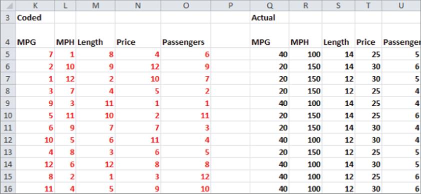
For example, the 7 in K5 in evconjoint.xlsx (to be selected by Solver) means “look up the attribute level for MPG in the 7^th row of B4:C15.” This yields 40 MPG in Q5. The formulas in Q5:U16 use a little known Excel function: the INDIRECT function. With this function a cell reference in an Excel formula after the word INDIRECT tells Excel to replace the cell reference with the contents of the cell. (If the contents of the cell are a range name, Excel knows to use the named range in the formula.) Therefore, copying the formula =VLOOKUP(K5,INDIRECT(Q$2),2,FALSE) from Q5:U16 translates the values 1–12 in K5:O16 into actual values of the attributes.

4. Next, in the cell range V5:W16 (see Figure 16.7), you can determine if a product profile represents an infeasible combination. Copy the formula =COUNTIFS(Q5,40,U5,6,S5,14) from V5 to V6:V16. This determines if the product profile is infeasible due to getting 40 MPG in a six-passenger 14-foot car. In a similar fashion Columns W and X yield a 1 if a product profile is infeasible for being either 14-foot, 150 MPH, and $20,000 price or 40 MPG with 150 MPH.

Figure 16-7: Excluding infeasible product profiles

5. Determine the correlations between each pair of attributes. A slick use of the INDIRECT function makes this easy: apply Create from Selection to the range Q4:U16 names Q5:Q16 MPG, R5:R16 MPH, and so on. Then, as shown in Figure 16.8, compute the absolute value of the correlation between each pair of attributes by copying the formula =ABS(CORREL(INDIRECT(O$19),INDIRECT($N20))) from O20 to O20:S24.

Figure 16-8: Correlations and target cell

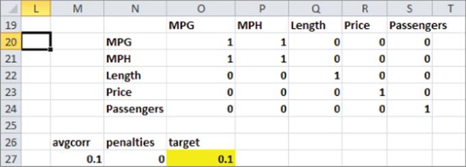
6. Now set up a target cell for Solver to minimize the sum of the average of the nondiagonal correlations (all diagonal correlations are 1) added to the number of infeasible product profiles. In cell M27 the formula =(SUM(O20:S24)-5)/20 calculates the average absolute value of the nondiagonal correlations. The target cell tries to minimize this average. This minimization moves you closer to an orthogonal design. Then determine the number of infeasible product profiles used in cell N27 with the formula =SUM(V5:X16). The final target cell is computed in cell O27 with the formula=N27+M27.

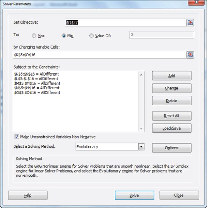
7. Finally, you are ready to invoke Solver! Figure 16.9 shows the Solver window. Simply change K5:O16 and invoke the AllDifferent option for each column. This ensures that columns K through O will contain the integers 1–12 once. In general, if you constrain a range of n cells to be AllDifferent, Excel ensures that these cells always assume the integer values 1, 2, …, n and each value will be used once. From the way you set up the formulas in Columns Q through U, this ensures that each level of all attributes appear the wanted number of times. After going to Evolutionary Solver options and resetting the Mutation rate to .5, you obtain the solution shown in Figures 16.7 and 16.8. Note that no infeasible product profiles occur, and all correlations except for MPH and MPG are 0. MPH and MPG have a correlation of –1 because the infeasible profiles force a low MPG to be associated with a large MPH, and vice versa.

Figure 16-9: Solver window for selecting product profiles

Developing a Conjoint Simulator

Conjoint analysis is often used to predict how the introduction of a new product (or changes in existing products) result in changes in product market share. These insights require the marketing analyst to develop a conjoint simulator that predicts how changes in product attributes change market share. This section illustrates how to calibrate a conjoint simulator to current share data and how to make predictions about how changes in products or the introduction of a new product can change market share. The work for this section is in the Segments worksheet of the conjoint.xls file and is shown in Figure 16.10.

Figure 16-10: Conjoint simulator

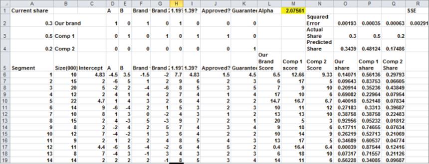
Suppose you're using cluster analysis (as shown in Chapter 23) and through a conjoint analysis the analyst has identified 14 market segments for a carpet cleaner. The regression equation for a typical member of each segment is given in the cell range D6:K19 and the size of each segment (in thousands) is the cell range B6:B19. For example, Segment 1 consists of 10,000 people and has Equation 1 as representative of consumer preferences for Segment 1. The range D2:K4 describes the product profile associated with the three products currently in the market. The brand currently has a 30 percent market share, Comp 1 has a 50 percent market share, and Comp 2 has a 20 percent market share.

To create a market simulator, you need to take the score that each segment associates with each product and translate these scores for each segment to a market share for each product. You can then calibrate this rule, so each product gets the observed market share. Finally, you can change attributes of the current products or introduce new products and “simulate” the new market shares for each product.

Consider Segment 1. Given that there are n products, you can assume the fraction of people in Segment 1 that will purchase Product i is given by the following:

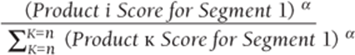
When you choose the value of , ensure that the predicted market share over all segments for each product matches as closely as possible the observed market share. To complete this process proceed as follows:

1. Copy the formula =SUMPRODUCT($D$2:$K$2,D6:K6)+C6 from L6 to L7:L19 to compute each segment's score for the product. Similar formulas in Columns M and N compute each segment's score for Comp 1 and Comp 2.

2. Copy the formula =L6^Alpha/($L6^Alpha+$M6^Alpha+$N6^Alpha) from O6 to the range O6:Q19 to compute for each segment the predicted market share for each product.

3. Copy the formula =SUMPRODUCT(O6:O19,$B$6:$B$19)/SUM($B$6:$B$19) from O4 to P4:Q4 to compute the predicted market share for each product by accounting for the size of each segment.

4. Copy the formula =(O4-O3)^2 from O2 to P2:Q2 to compute (based on the trial value of ) the squared error in trying to match the actual market share for each product.

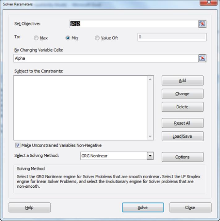
5. Use the Solver window, as shown in Figure 16.11, to yield the value of (2.08) that “calibrates” the simulator to actual market share data.

Figure 16-11: Solver window to calibrate conjoint simulator

Suppose you consider adding (with no price increase) a guarantee and believe you can obtain Good Housekeeping approval. In the worksheet GuaranteeApp you can change J2 and K2 to 1, and see that the conjoint simulator predicts that the market share will increase from 34 percent to 52 percent.

As an illustration of the use of a conjoint simulator, consider the problem of estimating the fraction of motorists who would use E-ZPass (an electronic method to collect tolls). Before New York and New Jersey implemented E-ZPass a conjoint simulator was used to choose the levels of the following attributes:

· Lanes available

· Method used to acquire E-ZPass

· Toll prices

· Other uses of E-ZPass

The conjoint simulator predicted that 49 percent of motorists would use E-ZPass. In reality, after seven years 44 percent of all motorists used E-ZPass.

Examining Other Forms of Conjoint Analysis

The approach to conjoint analysis thus far in this chapter involves using a set of a few (in the chapter example, five) product attributes to generate product profiles (in the chapter example, 18) which are ranked by a group of customers. Then multiple regression is used to rank the importance of the product attributes and rank the levels of each attribute. This approach to conjoint analysis is called full profile conjoint. The two shortcomings of full profile conjoint are as follows:

· Full profile conjoint has difficulty dealing with many attributes because the number of profiles that must be ranked grows rapidly with the number of attributes.

· Consumers have difficulty ranking product profiles. Rather than having a consumer rank product profiles, it is much easier for a consumer to choose the best available option.

This section provides a brief description of two alternate forms of conjoint analysis: adaptive/hybrid conjoint analysis and choice-based conjoint analysis, which attempt to resolve the problems with full profile conjoint analysis.

Adaptive/Hybrid Conjoint Analysis

If a product has many attributes, the number of product profiles needed to analyze the relative importance of the attributes and the desirability of attribute levels may be so large that consumers cannot accurately rank the product profiles. In such situations adaptive or hybrid conjoint analysis(developed by Sawtooth Software in 1985) may be used to simplify the consumer's task.

In step 1 of an adaptive conjoint analysis, the consumer is asked to rank order attribute levels from best to worst. In step 2 the consumer is asked to evaluate the relative desirability of different attribute levels. Based on the consumer's responses in steps 1 and 2 (this is why the method is called adaptive conjoint analysis), the consumer is asked to rate on a 1–9 scale the strength of his preference for one product profile over another. If, for example, a consumer preferred Design A to Design B and Brand 1 to Brand 2, the adaptive conjoint software would never create a paired comparison between a product with Design A and Brand 1 to Design B and Brand 2 (all other attributes being equal).

Choice-Based Conjoint Analysis

In choice-based conjoint analysis, the consumer is shown several product profiles and is not asked to rank them but simply to state which profile (or none of the available choices) she would choose. This makes the consumer's task easier, but an understanding of choice-based conjoint analysis requires much more mathematical sophistication then ordinary conjoint analysis. Also, choice-based conjoint analysis cannot handle situations in which attributes such as price or miles per gallon for a car are allowed to assume a range of values. In Chapter 18 you will learn about the theory ofdiscrete choice, which is mathematically more difficult than multiple linear regression. Discrete choice generalizes choice-based conjoint analysis by allowing product attributes to assume a range of values.

Summary

In this chapter you learned the following:

· Conjoint analysis is used to determine the importance of various product attributes and which levels of the attributes are preferred by the customer.

· In full profile conjoint analysis, the consumer is asked to rank a variety of product profiles.

· To make the estimates of each attribute's importance and level preferences more accurate, it is usually preferable to make the correlation between any pair of attributes in the product profiles close to 0.

· Multiple linear regression (often using dummy variables) can easily be used to rank the importance of attributes and the ranking of levels within each attribute.

· A conjoint simulator can predict how changes in existing products (or introduction of new products) will change product market shares.

· Adaptive/hybrid conjoint analysis is often used when there are many product attributes. After having the consumer answer questions involving ranking attributes and levels, the software adapts to the consumer's preferences before asking the consumer to make paired comparisons between product profiles.

· Choice-based conjoint analysis ascertains the importance of attributes and the ranking of levels within each attribute by asking the consumer to simply choose the best of several product profiles choices (usually including an option to choose none of the available product profiles.) The extension of choice-based conjoint analysis to a situation where an attribute such as price is continuous is known as discrete choice and will be covered in Chapter 18.

Exercises

1. Determine how various attributes impact the purchase of a car. There are four attributes, each with three levels:

· Brand: Ford = 0, Chrysler = 1, GM = 2

· MPG: 15 MPG = 0, 20 MPG = 1, 25 MPG = 2

· Horsepower (HP): 100 HP = 0, 150 HP = 1, 200 HP = 2

· Price: $18,000 = 0, $21,000 = 1, $24,000 = 2

The nine product profiles ranked in Figure 16.12 were evaluated by a consumer.

Figure 16-12: Auto data for Exercise 1

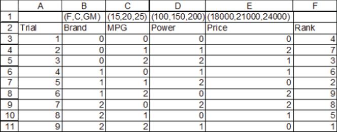
(a) For this market segment, rank the product attributes from most important to least important.

(b) Consider a car currently getting 20 MPG selling for $21,000. If you could increase MPG by 1 mile, how much could you increase the price of the car and keep the car just as attractive to this market segment?

(c) Is this design orthogonal?

NOTE

When you run the regression in Excel, you can obtain a #NUM error for the p-values. You still may use the Coefficients Column to answer the exercise.

2. The soda.xlsx file (see Figure 16.13) gives a consumer's ranking on an orthogonal design with 12 product profiles involving a comparison of Coke and Pepsi. The attributes and levels are as follows:

· Brand: Coke or Pepsi

· Packaging: 12 oz. can or 16 oz. bottle

· Price per ounce: 8 cents, 10 cents, 12 cents

· Calories per ounce: 0 or 15

Figure 16-13: Soda data for Exercise 2

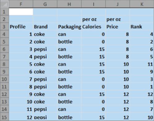
Determine the ranking of the attributes' importance and the ranking of all attribute levels.

3. Show that the list of product profiles in the following table yields an orthogonal design.