Marketing Analytics: Data-Driven Techniques with Microsoft Excel (2014)

Part IV. What do Customers Want?

Chapter 18. Discrete Choice Analysis

In Chapter 16, “Conjoint Analysis,” you learned how the marketing analyst could use a customer's ranking of product profiles to determine the relative importance the customer attaches to product attributes and how a customer ranks the level of each product attribute. In this chapter you will learn how to use discrete choice analysis to determine the relative importance the customer attaches to product attributes and how a customer ranks the level of each product attribute. To utilize discrete choice analysis, customers are asked to make a choice among a set of alternatives (often including none of the given alternatives). The customer need not rank the product attributes. Using maximum likelihood estimation and an extension of the logit model described in Chapter 17, “Logistic Regression,” the marketing analyst can estimate the ranking of product attributes for the population represented by the sampled customers and the ranking of the level of each product attribute.

In this chapter you learn how discrete choice can be used to perform the following:

· Estimate consumer preferences for different types of chocolate.

· Estimate price sensitivity and brand equity for different video games, and determine the profit maximizing price of a video game.

· Model how companies should dynamically change prices over time.

· Estimate price elasticity.

· Determine the price premium a national brand product can command over a generic product.

Random Utility Theory

The concept of random utility theory provides the theoretical basis for discrete choice analysis. Suppose a decision maker must choose among n alternatives. You can observe certain attributes and levels for each alternative.

The decision maker associates a utility U_j with the jth alternative. Although the decision maker knows these utilities, the marketing analyst does not. The random utility model assumes the following:

Here V_j is a deterministic “score” based on the levels of the attributes that define the alternative, and the ε_j 's are random unobservable error terms. The decision maker is assumed to choose the alternative j (j = 1, 2, …, n) having the largest value of U_j. Daniel McFadden showed (see “Conditional Logit Analysis of Qualitative Choice Behavior” in Frontiers of Econometric Behavior, Academic Press, 1974) that if the ε_j 's are independent Gumbel (also known as extreme value) random variables, each having the following distribution function: F(x)=Probability ε_j <= x)= e^-e-x, then the probability that the decision maker chooses alternative j (that is, U_j = max_{k=1,2,,....,n}U_k) is given by the following:

1

Of course, Equation 1 is analogous to the logit model of Chapter 17 and is often called the multinomial logit model. Equation 1 is of crucial importance because it provides a reasonable method for transforming a customer's score for each product into a reasonable estimate of the probability that the person will choose each product. In the rest of this chapter you will be given the alternative chosen by each individual in a set of decision makers. Then you use Equation 1 and the method of maximum likelihood (introduced in Chapter 17) to estimate the importance of each attribute and the ranking of the levels within each attribute.

NOTE

If this discussion of random utility theory seems too technical, do not worry; to follow the rest of the chapter all you really need to know is that Equation 1 can be used to predict the probability that a decision maker chooses a given alternative.

NOTE

Another commonly used assumption is that the errors in Equation 1 are not independent and have marginal distributions that are normal. This assumption can be analyzed via probit regression, which is beyond the scope of this book. In his book Discrete Choice Methods with Simulation, 2nd ed. (Cambridge University Press, 2009), Kenneth Train determined how changes in the price of different energy sources (gas, electric, and so on) affect the fraction of homes choosing different sources of energy. You can refer to his book for an extensive discussion of probit regression.

Discrete Choice Analysis of Chocolate Preferences

Suppose that eight alternative types of chocolate might be described by the levels of the following attributes:

· Dark or milk

· Soft or chewy

· Nuts or no nuts

The eight resulting types of chocolate are listed here:

· Milk, chewy, no nuts

· Milk, chewy, nuts

· Milk, soft, no nuts

· Milk, soft, nuts

· Dark, chewy, no nuts

· Dark, chewy, nuts

· Dark, soft, no nuts

· Dark, soft, nuts

Ten people were asked which type of chocolate they preferred. (People were not allowed to choose none of the above.) The following results were obtained:

· Two people chose milk, chewy, nuts.

· Two people chose dark, chewy, no nuts.

· Five people chose dark, chewy, nuts.

· One person chose dark, soft, nuts.

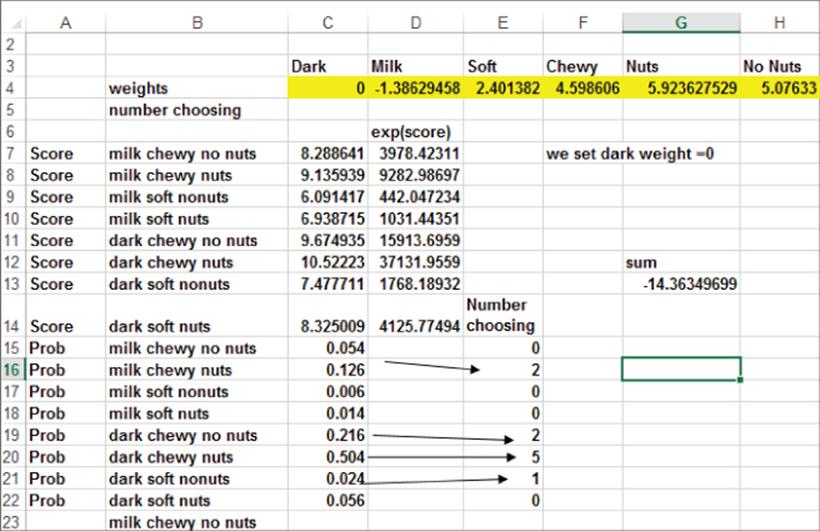
You can use discrete choice analysis to determine the relative importance of the attributes and, within each attribute, rank the levels of the attributes. The work for this process is shown in Figure 18.1 and is in the chocolate.xls file.

Figure 18-1: Chocolate discrete choice example

Assume the score for each of the eight types of chocolate will be determined based on six unknown numbers which represent the “value” of various chocolate characteristics.

· Value for dark

· Value for milk

· Value for soft

· Value for chewy

· Value for nuts

· Value for no nuts

The score, for example of milk, chewy, no nuts chocolate, is simply determined by the following equation:

2

To estimate the six unknowns proceed as follows:

1. In cells C4:H4 enter trial values for these six unknowns.

2. In cells C7:C14 compute the score for each type of chocolate. For example, in C7 Equation 2 is used to compute the score of milk, chewy, no nuts with the formula =D4+F4+H4.

3. Use Equation 1 to compute the probability that a person will choose each of the eight types of chocolate. To do so copy the formula =EXP(C7) from D7 to D8:D14 to compute the numerator of Equation 1 for each type of chocolate. Then copy the formula =D7/SUM($D$7:$D$14) from C15 to C16:C22 to implement Equation 1 to compute the probability that a person will choose each type of chocolate.

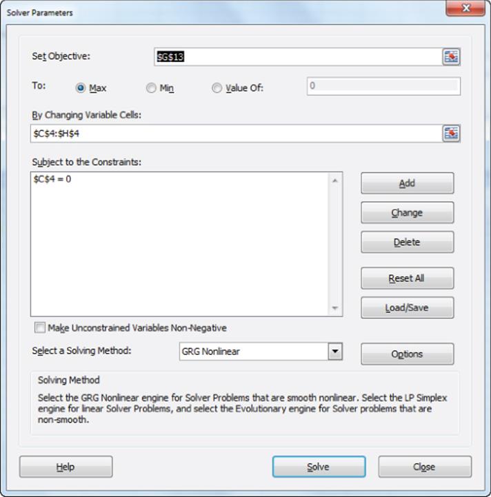
4. Use the technique of maximum likelihood (actually maximizing the logarithm of maximum likelihood) to determine the six values that maximize the likelihood of the observed choices. Note that Equation 2 implies that if you add the same constant to the score of each alternative, then for each alternative the probabilities implied by Equation 2 remain unchanged. Therefore when you maximize the likelihood of the observed choices, there is no unique solution k. Therefore you may arbitrarily set any of the changing cells to 0. For this example suppose the value of dark = 0.

The likelihood of what you have observed is given by the following equation:

3

Essentially you find the likelihood of what has been observed by taking the probability of each selected alternative and raising it to a power that equals the number of times the selected alternative is observed. For example, in the term (P of D,C,N)⁵, (P of D,C,N) is raised to the fifth power because five people preferred dark and chewy with nuts.

Equation 3 uses the following abbreviations:

· P = Probability

· M = Milk

· D = Dark

· N = Nuts

· NN = No Nuts

· C = Chewy

· S = Soft

Recall the following two basic laws of logarithms:

4

5

You can apply Equations 4 and 5 to Equation 3 to show that the natural logarithm of the likelihood of the observed choices is given by the following equation:

6

Cell G13 computes the Log Likelihood with the formula =E16*LN(C16)+E19*LN(C19)+E20*LN(C20)+E21*LN(C21).

You can use the Solver window in Figure 18.2 to determine the maximum likelihood estimates of the values for each level of each attribute. The values enable you to determine the importance of each attribute and the rankings within each attribute of the attribute levels.

Figure 18-2: Solver window for chocolate example

Refer to Figure 18.1 and you can find the following maximum likelihood estimates:

· Dark = 0, Milk = −1.38, so Dark is preferred to Milk overall and the difference between the Dark and Milk values is 1.38.

· Chewy = 4.59 and Soft = 2.40, so Chewy is preferred to Soft overall and the difference between the Chewy and Soft scores is 2.19.

· Nuts = 5.93 and No Nuts = 5.08, so Nuts is preferred to No Nuts and the difference between the Nuts and No Nuts scores is 0.85.

You can rank the importance of the attributes based on the difference in scores within the levels of the attribute. This tells you that the attributes in order of importance are Chewy versus Soft, Dark versus Milk, and Nuts versus No Nuts. This is consistent with the fact that nine people prefer Chewy, eight prefer Dark, and seven prefer Nuts.

Incorporating Price and Brand Equity into Discrete Choice Analysis

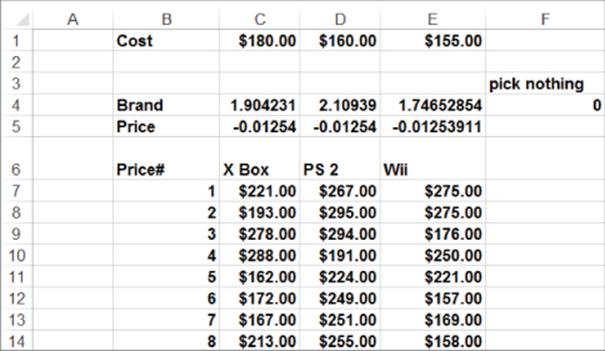
In this section you learn how to incorporate price and brand equity into a discrete choice analysis. The first model is in the file Xbox1.xls and the data is shown in Figure 18.3.

Figure 18-3: Video game data

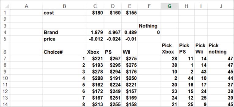
The data indicates that 100 people were shown eight price scenarios for Xbox, PlayStation (PS), and Wii. Each person was asked which product they would buy (or none) for the given prices. For example, if Xbox sold for $221, PS for $267, and Wii for $275, 28 people chose Xbox, 11 chose PS, 14 chose Wii, and 47 chose to buy no video game console. You are also given the cost to produce each console.

You will now learn how to apply discrete choice analysis to estimate price sensitivity and product brand equity in the video game console market. For each possible product choice, assume the value may be computed as follows:

· Value Xbox = Xbox brand weight + (Xbox price) * (Xbox price sensitivity)

· Value PS = PS brand weight + (PS price) * (PS price sensitivity)

· Value Wii = Wii brand weight + (Wii price) * (Wii price sensitivity)

· Assume Weight for Nothing = 0, so Value Nothing = 0

Now you can use maximum likelihood estimation to estimate the brand weight for each product and the price sensitivity for each product. The strategy is to find the Log Likelihood of the data for each set of prices, and then, because of Equation 4, add the Log Likelihoods. By maximizing the Log Likelihood you can obtain the set of weights that maximize the chance to observe the actual observed choice data. The work is shown in Figure 18.4. Proceed as follows:

1. In C4:E5 enter trial values for brand coefficients and price sensitivities for each product. In F4 set the Nothing “brand” coefficient equal to 0.

2. Copy the formula =C$4+C$5*C7 from K7 to K7:M14 to generate scores for each product for each scenario.

3. Copy the formula =$F$4 from N7 to N7:N14 to generate for each scenario the score for no purchase.

4. Copy the formula =EXP(K7)/(EXP($K7)+EXP($L7)+EXP($M7)+EXP($N7)) from O7 to O7:R14 to utilize Equation 1 to compute for each price scenario the probability that each product (or no purchase) is chosen.

5. To see how to compute the likelihood of the observed results for each scenario, note that in the first scenario the likelihood is as follows:

The goal is to maximize the sum of the logarithms of the likelihoods for each scenario. For the first scenario the logarithm of the likelihood is as follows:

This follows from Equations 4 and 5. Therefore copy the formula G7*LN(O7)+H7*LN(P7)+I7*LN(Q7)+J7*LN(R7) from S7 to S7:S14 to compute the logarithm of the likelihood for each scenario.

6. In cell S5 you can create the target cell needed to compute maximum likelihood estimates for the changing cells (the range C4:E5 and F4). The target cell is computed as the sum of the Log Likelihoods with the formula =SUM(S7:S14).

7. Use the Solver window shown in Figure 18.5 to determine the brand weights and price sensitivities that maximize the sum of the Log Likelihoods. This is equivalent, of course, to maximizing the likelihood of the observed choices given by Equation 3. Note that you constrained the score for the Nothing choice to equal 0 with the constraint $F$4 = 0.

Figure 18-4: Maximum likelihood estimation for video console example

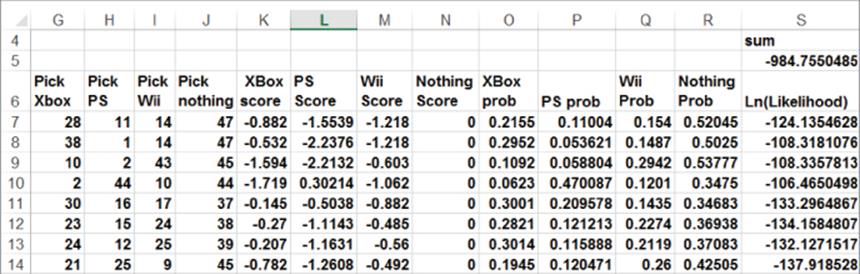
Figure 18-5: Solver window for maximum likelihood estimation

The weights and price sensitivities are shown in the cell range C4:E5 of Figure 18.3. At first glance it appears that PS has the highest brand equity, but because PS also has the most negative price sensitivity, you are not sure. In the “Evaluating Brand Equity” section you constrain each product's price weight to be identical so that you can obtain a fair comparison of brand equity for each product.

Pricing Optimization

After you have estimated the brand weights and price sensitivities, you can create a market simulator (similar to the conjoint simulator of Chapter 16) to help a company price to maximize profits. Suppose you work for Xbox and want to determine a profit maximizing price. Without loss of generality, assume the market consists of 100 customers. Then your goal is to price Xbox to maximize profit earned per 100 customers in the market. Make the following assumptions:

· Xbox price is $180.

· PS price is $215 and Wii price is $190.

· Each Xbox purchaser buys seven games.

· Xbox sells each game for $40 and buys each game for $30.

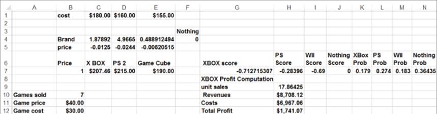
To determine what price maximizes profit from Xbox look at the worksheet pricing in file Xbox1.xls (also shown in Figure 18.6).

Figure 18-6: Determining Xbox price

Proceed as follows:

1. To perform the pricing optimization you only need one row containing probability calculations from the model worksheet. Therefore in Row 7 of the pricing worksheet recreate Row 7 from the model worksheet. Also insert a trial price for Xbox in C7, and enter information concerning Xbox in B10 and B11.

2. In cell H9, compute unit sales of Xbox with the formula =100*K7.

3. In cell H10, compute Xbox revenue from consoles and games with the formula =C7*H9+H9*B10*B11.

4. In cell H11, enter the cost of Xbox consoles and games with the formula =H9*C1+B10*H9*B12.

5. In cell H12, compute the profit with the formula =H10-H11.

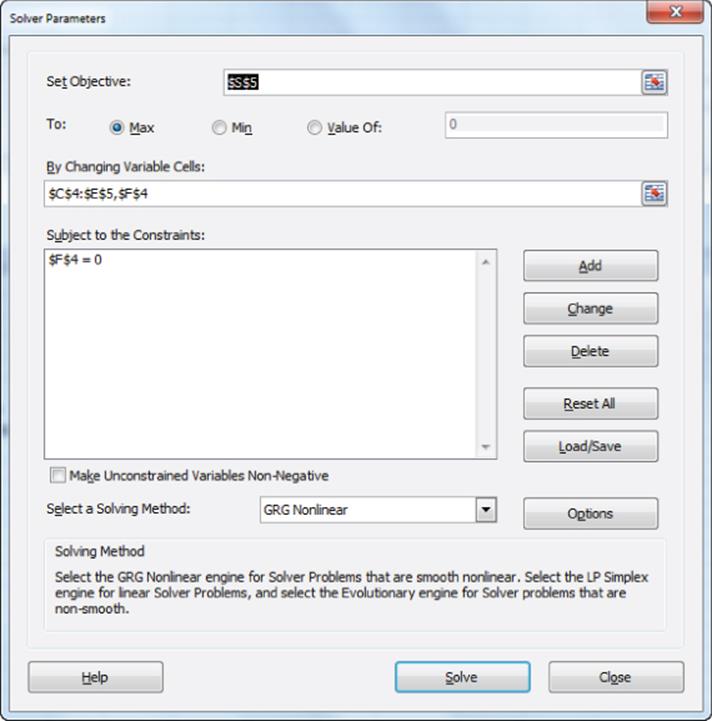
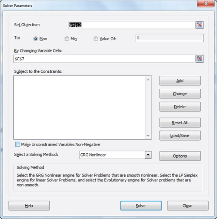
6. Use the Solver window in Figure 18.7 to yield a profit-maximizing price of $207.47 for Xbox.

Figure 18-7: Solver window for Xbox price

Evaluating Brand Equity

Based on the pricing analyses performed in the previous section, you can also estimate the value of each brand, or brand equity, by forcing the price weight to be identical across all competitors. For instance, you might say PS has the largest brand equity because its brand coefficient is the largest. As previously pointed out, however, PS has the most negative price weight, so it is not clear that PS has the largest brand equity. For example, if PS had the largest brand equity then you would think that the scores and choice mechanism would indicate that the market would prefer a PS over an Xbox or Wii at a $200 price. Due to the large negative price coefficient for PS, it is unclear whether PS would be preferred if all products sold for the same price. To correctly determine brand equity, you must rerun the Solver model assuming that the price weight is the same for each product. Setting the price weights equal for all products ensures that if all products sell for the same price the market would prefer the product with the largest brand weight. The results are in the worksheet Brand equity and price of workbook Xbox2.xls, and the changes from the previous model are shown in Figure 18.8. Set D5 and E5 equal to C5, and delete D5 and E5 as changing cells. After running Solver, you find that PS has the largest brand equity, followed by Xbox and Wii.

Figure 18-8: PS has the largest brand equity

Testing for Significance in Discrete Choice Analysis

Once you have estimated the brand values and price weights, you can plug the product prices into Equation 2 and forecast market shares. You might wonder whether including a factor such as price in market share forecasts improves the quality of the forecasts. To determine whether or not adding a factor such as price to a discrete choice analysis significantly improves the model's predictions for product market shares, proceed as follows:

1. Let LL(Full) = Log Likelihood when all changing cells are included.

2. Let LL(Full –q) = Log Likelihood when changing cell q is omitted from the model.

3. Let DELTA(q) = 2 * (LL(FULL) –LL(FULL –q)). Then DELTA(q) follows a Chi-Square random variable with 1 degree of freedom, and a p-value for the significance of q may be computed with the Excel formula =CHIDIST(DELTA(q),1).

4. If this formula yields a p-value less than .05, you may conclude that the changing cell q is of significant use (after adjusting for other changing cells in the model) in predicting choice.

You can use this technique to test if incorporating price in your choice model is a significant improvement over just using the brand weights. In the Brand Equity and Price worksheet of workbook Xbox2.xls, you can find LL(Full Model) = −996.85. In worksheet Brand equity and price the model is run with the price weight set to 0, which obtains LL(Model(no price) = −1045.03. Then Delta(q) = 96.37 and CHIDIST(96.37,1) = 10^-22. It is therefore virtually certain that price is a significant factor in the choice of a video game console.

Dynamic Discrete Choice

Although the previous sections and analyses offer important insights regarding the drivers of consumer choice, as well as pricing and brand equity implications, they do not represent the “real world” in the sense that the previous analyses do not address competitive dynamics. In the real world, if one firm changes its price, it should expect competitors to react. This section addresses competitive dynamics in discrete choice analysis.

If Xbox sets a price of $207 as recommended previously, then PS and Wii would probably react by changing their prices. In this section you will learn how to follow through the dynamics of this price competition. Usually one of two situations occurs:

· A price war in which competitors continually undercut each other

· A Nash equilibrium in which no competitor has an incentive to change its price. Nash equilibrium implies a stable set of prices because nobody has an incentive to change their price.

The file Xbox3.xls contains the analysis. The model of competitive dynamics is shown in Figure 18.9.

1. To begin, copy the formulas in H9:H12 to I9:J12. This computes profit for PS and Wii, respectively.

2. Change Solver to maximize I12 by changing D7. The resulting Solver solution shows that PS should now charge $173.55.

3. Next, change the target cell to maximize J12 by changing E7. The resulting Solver solution shows that given current prices of other products, Wii should charge $260.74.

4. Now it is Xbox's turn to change the Xbox price: maximize H12 by changing C7. Xbox now sells for $202.38. Repeating the process, you find that prices appear to stabilize at the following levels:

· Xbox: $202.64

· PS: $175.18

· Wii: $260.94

Figure 18-9: Dynamic pricing of Video game consoles

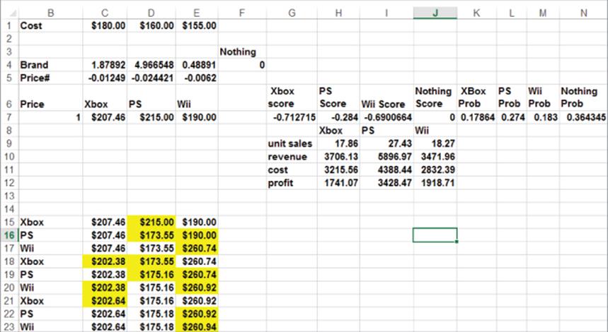
With this set of prices, no company has an incentive to change its price. If it changes its price, its profit will drop. Thus you have found a stable Nash equilibrium.

Independence of Irrelevant Alternatives (IIA) Assumption

Discrete choice analysis implies that the ratio of the probability of choosing alternative j to the chance of choosing alternative i is independent of the other available choices. This property of discrete choice modeling is called the Independence of Irrelevant Alternatives (IIA) assumption. Unfortunately, in many situations you will learn that IIA is unreasonable.

From Equation 2 you can show (see Exercise 6) that for any two alternatives i and j, Equation 7 holds.

7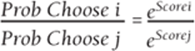

Equation 7 tells you that the ratio of the probability of choosing alternative i to the probability of choosing alternative j is independent of the other available choices. This property of discrete choice modeling is called the Independence of Irrelevant Alternatives (IIA) assumption. The following paradox (called the Red Bus/Blue Bus Problem) shows that IIA can sometimes result in unrealistic choice probabilities.

Suppose people have two ways to get to work: a Blue Bus or a Car. Suppose people equally like buses and cars so the following is true:

Now add a third alternative: a Red Bus. Clearly the Red and Blue Buses should divide the 50-percent market share for buses and the new probabilities should be:

· Probability Car = 0.5

· Probability Blue Bus = 0.25

· Probability Red Bus = 0.25

The IIA assumption implies that the current ratio of Probability Blue Bus/Probability Car will remain unchanged. Because Probability Red Bus = Probability Blue Bus, you know that discrete choice will produce the following unrealistic result:

· Probability Car = 1/3

· Probability Blue Bus = 1/3

· Probability Red Bus = 1/3

The IIA problem may be resolved by using more advanced techniques including mixed logit, nested logit, and probit. See Train (2009) for details.

Discrete Choice and Price Elasticity

In Chapter 4, “Estimating Demand Curves and Using Solver to Optimize Price,” you learned that a product's price elasticity is the percentage change in the demand for a product resulting from a 1 percent increase in the product's price. In this section you will learn how discrete choice analysis can be used to estimate price elasticity. Define the following quantities as indicated:

· Prob(j) = Probability product j is chosen.

· Price(j) = Price of product j.

· β (j) = Price coefficient in score equation.

From Equation 2 it can be shown that:

8

The cross elasticity (call it E(k,j)) of product k with respect to product j is the percentage change in demand for product k resulting from a 1 percent increase in the price of product j. From Equation 2 it can be shown that:

9

NOTE

All products other than product j have the same cross elasticity. This is known as the property of uniform cross elasticity.

The file Xbox4.xls illustrates the use of Equations 8 and 9. Return to the video game example and assume that the current prices are Xbox = $200, PS = $210, and Wii = $220, as shown in Figure 18.10.

Figure 18-10: Elasticities for Xbox example

The price elasticity for Xbox is −1.96 (a 1 percent increase in Xbox price reduces Xbox sales by 1.96 percent) and the cross elasticities for Xbox price are .55. (A 1 percent increase in Xbox price increases demand for other products by 0.55 percent)

Summary

In this chapter you learned the following:

· A discrete choice analysis helps the marketing analyst determine what attributes matter most to decision makers and how levels of each attribute are ranked by decision makers.

· To begin a discrete choice analysis, decision makers are shown a set of alternatives and asked to choose their most preferred alternative.

· The analyst must determine a model that is used to “score” each alternative based on the level of its attributes.

· The fraction of decision makers that choose alternative j is assumed to follow the multinomial logit model:

1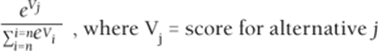

· Maximum Likelihood is used to estimate the parameters (such as brand equity and price sensitivity) in the scoring equation.

· In a discrete analysis, a Chi Square Test based on the change in the Log Likelihood Ratio can be used to assess the significance of a changing cell.

· The Independence of Irrelevant Alternatives (IIA) that follows from Equation 2 implies that the ratio of the probability to choose alternative i to the probability to choose alternative j is independent of the other available choices. In situations like the Red Bus/Blue Bus example, discrete choice analysis may lead to unrealistic results.

· The multinomial logit version of discrete choice enables you to easily compute price elasticities using the following equations:

(8) Price Elasticity for Product j = (1 – Prob(j)) * Price(j) * β (j)

(9) E(k,j) = − Prob(j) * Price(j) * β (j)

Exercises

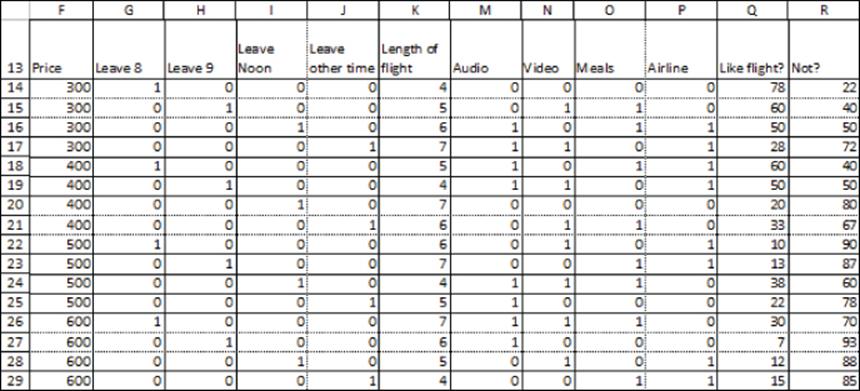
1. In her book Discrete Choice Modeling and Air Travel Demand (Ashgate Publishing, 2010), Per Laurie Garrow details how airlines have predicted how changes in flight prices will affect their market share. Use this example to perform some similar analysis. Delta Airlines wants to determine the profit maximizing price to charge for a 9 a.m. New York to Chicago flight. A focus group has been shown 16 different flights and asked if it would choose a flight if the flight were available. The results of the survey are in file Airlinedata.xlsx, and a sample is shown in Figure 18.11. For example, when shown a Delta 8 a.m., four-hour flight with no music (audio), video, or meals, priced at $300, 78 people chose that flight over choosing not to take a flight at all (Delta = 0, United = 1).

Figure 18-11: Data for Exercise 1

(a) Which airline (Delta or United) has more brand equity on this route?

(b) Delta wants to optimally design a 9 a.m. flight. The flight will have audio and take six hours. There are 500 potential flyers on this route each day. The plane can seat at most 300 people. Determine the profit maximizing price, and whether Delta should offer a movie and/or meals on the flight. The only other flight that day is a $350 United 8 a.m., five-hour flight with audio, movies, and no meals. Delta's cost per person on the flight breaks down as follows:

Help Delta maximize its profit on this flight.

2. P&G is doing a discrete choice analysis to determine what price to charge for a box of Tide. It collected the data shown in Figure 18.12. For example, when people were asked which they prefer: Generic for $5, Tide for $8, or None, 35 people said generic, 22 picked Tide, and 43 chose None.

Using a discrete choice model with the same price weight for each product, answer the following questions:

Figure 18-12: Data for Exercise 2

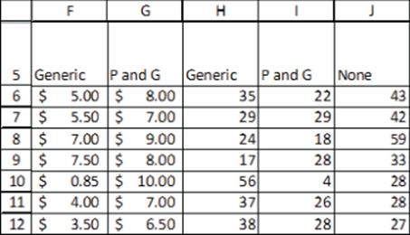
(a) Using the value-based approach to pricing outlined in Chapter 16, “Conjoint Analysis,” what price premium can Tide command over the generic product?

(b) If the generic product sold for $5, what price would you recommend for Tide?

3. P&G wants to determine if it should introduce a new, cheaper version of Head and Shoulders shampoo. It asked a focus group which of three products it would prefer at different prices (see Figure 18.13). For example, if all three products cost $3.60, 70 people prefer Head and Shoulders, 13 prefer Head and Shoulders Lite, 4 prefer CVS, and 13 would buy no dandruff shampoo.

Figure 18-13: Data for Exercise 3

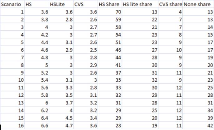
(a) Use this data to calibrate a discrete choice model. Use the same price weight for each product.

(b) Suppose the CVS shampoo sells for $3.00. If the unit cost to produce Head and Shoulders is $2.20 and the unit cost to produce Head and Shoulders Lite is $1.40, what pricing maximizes P&G's profit?

(c) By what percentage does the introduction of Head and Shoulders Lite increase P&G's profit?

4. CVS wants to determine how to price Listerine with whitener (LW), Listerine (LIST), and CVS mouthwash. One hundred people were shown the following price scenarios, and their choices are listed in Figure 18.14. For example, with LW at $6.60, LIST at $5, and CVS at $3.25, 37 picked no mouthwash, 18 chose LISTW, 20 preferred LIST, and 25 chose CVS.

Figure 18-14: Data for Exercise 4

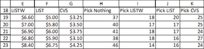
(a) Fit a discrete choice model to this data. Use only a single price variable.

(b) Using Value-Based Pricing, estimate the value customers place on the whitening feature.

(c) Using Value-Based Pricing, estimate the brand equity of P&G.

NOTE

LIST and CVS have the same features; the only difference is the name on the bottle.

(d) Suppose the price of CVS mouthwash must be $6. Also assume CVS pays $4 for a bottle of LISTW, $3 for a bottle of LIST, and $2.50 for a bottle of CVS. What price for LISTW and LIST maximizes profits for CVS?

5. Armed Forces recruiting has asked for your help to allocate recruiting bonuses among the Air Force, Navy, and Army. During the next year, 1,000,000 people are expected to show interest in enlisting. The United States needs 100,000 enlistees in the Air Force and Navy and 250,000 enlistees in the Army. Recruiting bonuses of up to $30,000 are allowed. A discrete choice study has been undertaken to determine the minimum cost recruiting budget that will obtain the correct number of enlistees. The information shown in Figure 18.15 is available:

For example, 100 potential recruits were offered $10,000 to enlist in each service. Fifty-nine chose not to enlist, 25 chose the Air Force, 10 chose the Navy, and 6 chose the Army.

Figure 18-15: Data for Exercise 5

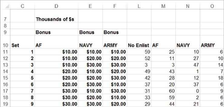
(a) Develop a discrete choice model that can determine how the size of the bonuses influences the number of recruits each service obtains. Assume the following:

Use the same bonus weight for each service.

(b) Assuming the bonus for each service can be at most $30,000, determine the minimum cost bonus plan that will fill the U.S. recruiting quotas.

6. Verify Equation 7.