Marketing Analytics: Data-Driven Techniques with Microsoft Excel (2014)

Part V. Customer Value

Chapter 21. Customer Value, Monte Carlo Simulation, and Marketing Decision Making

In many situations the results of a marketing decision are highly uncertain. For example, when Land's End mails a catalog, it does not know how many dollars of profit will be generated by the catalog. The profit generated on a mailing often depends on the customer's past response to catalog mailings. Likewise, consider a merchant who is considering using a Groupon offer. The amount of profit or loss obtained is uncertain because it depends on the number of people taking the offer who become loyal customers as well as the long-term value generated by the customers. Monte Carlo simulation is a method for determining the range of outcomes that can occur in a situation. Using Monte Carlo simulation you may find that a Groupon offer has a 90 percent chance of earning a profit.

In this chapter you learn how combining Monte Carlo simulation and the concept of long-term customer value can improve a company's decision making by allowing the marketer to estimate the range of outcomes that can result from a marketing decision.

A Markov Chain Model of Customer Value

Often a customer passes through various stages of a customer life cycle. For example, a Progressive car insurance policy holder may start as a teenager who has several accidents and turn into a 30-year-old who never has another accident. A Land's End catalog customer may begin as someone who bought a sweater last month and turn into someone who has not made another purchase in the last two years.

The value of a customer therefore depends on where the customer is currently in this life cycle. Calculating customer value based on this cycle can be achieved using Monte Carlo simulation. Monte Carlo simulation is a method to model uncertainty and estimate a range of outcomes under uncertainty by replaying a situation out many times (even millions of times). Monte Carlo simulation began during World War II when scientists tested to see if the random neutron diffusion in the nuclear fission involved in the atomic bomb would actually result in a bomb that worked. Mathematicians James von Neumann and Stanislaw Ulam the simulation procedure named Monte Carlo after the gambling casinos in Monaco. As you will learn, Monte Carlo simulation bears a resemblance to repeatedly tossing “electronic dice” or repeatedly spinning an “electronic roulette wheel.”

The following example shows how you can use Monte Carlo simulation to model customer value in situations in which customers pass through stages.

Imagine that a small mail-order firm mails out catalogs every three months (at a cost of $1). Based on analyses performed on historical purchase data (probably using PivotTables!), the marketing analyst found that each time a customer places an order, the profit earned (exclusive of mailing cost) follows a normal random variable with mean $60 and standard deviation $10. The probability that a customer orders from a catalog depends on recency (number of catalogs since last order) and frequency (total number of orders placed), as shown in Figure 21.1.

Figure 21-1: Chance of purchasing from Land's End catalog

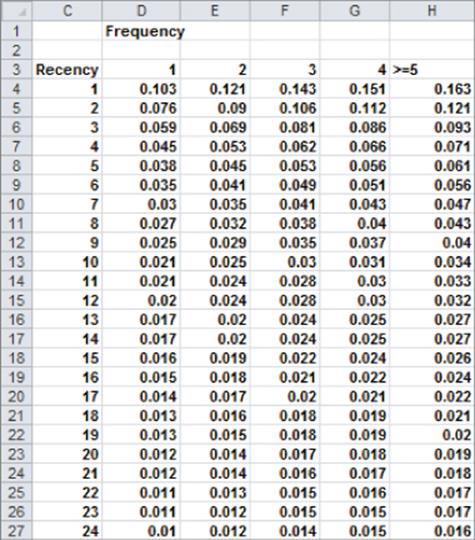
For example, based on the preceding analysis, a customer (call her Miley) who has ordered twice and whose last order was three catalogs ago has a 6.9 percent chance of ordering. This assumes that a customer's future evolution depends only on her present state. For example, in analyzing Miley's future purchases you need only know she has ordered twice and her last order was three catalogs ago. You do not need to know, for example, the timing of other orders that were placed before the last order. This model is an example of a Markov Chain. In a Markov Chain a process evolves from one state to another state, with the probability of going to the next state depending only on the current state. In this example the customer's current state is the number of periods in the past when last order occurred and the number of previous orders. Given this information you can determine how the value of a customer who has ordered once depends on recency.

Assume you stop mailing to a customer after she fails to order 24 consecutive times. Also assume the annual discount rate (often called the weighted average cost of capital [WACC]) is 3 percent per period (or 1.03⁴) per year. The following steps describe how to determine the customer value for a customer who has bought one time (frequency = 1) and bought from the last received catalog (recency = 1). The work for this example is in the Markov.xls file (see Figure 21.2).

1. In cell C30 enter the recency level (in this case 1) with the formula =Initial_recency.

2. In cell D30 enter the initial frequency with the formula =Original_Frequency.

3. In cell E30 determine the probability that the customer orders in with the formula =IF(B30="no",0,INDEX(probs,C30,D30)). If you have ended the relationship with the customer, the order probability is 0.

Figure 21-2: Land's End Customer Value model

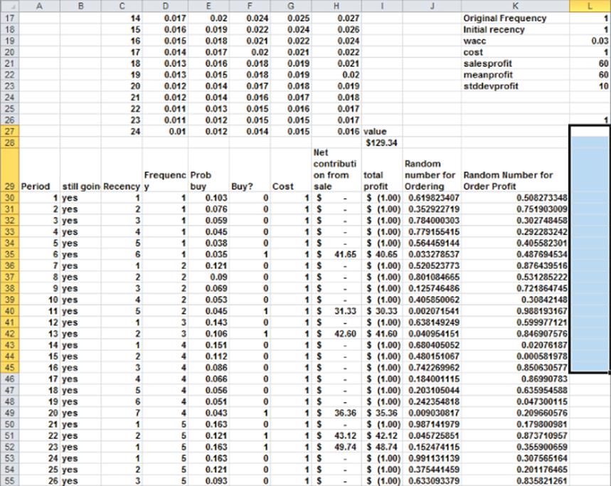
The key to performing a Monte Carlo simulation is the RAND() function. When you enter the RAND() function in a cell, Excel enters a number that is equally likely to assume any value greater than 0 and less than 1. For example, there is a 10 percent chance that a number less than or equal to 0.10 appears in a cell; a 30 percent chance that a number greater than or equal to 0.4 and less than or equal to 0.7 appears in the cell; and so on. Values in different cells containing a RAND() function are independent; that is, the value of a RAND() in one cell does not have influence on the value of a RAND()in any other cell. In a Monte Carlo simulation, you use RAND() functions to model sources of uncertainty. Then you recalculate the spreadsheet many times (say 10,000) to determine the range of outcomes that can occur. The RAND() function plays the role of “electronic dice.”

During each three-month period, the Monte Carlo simulation uses two RAND() functions. One RAND() determines if the customer places an order. If the customer orders, the second RAND() function determines the profit (excluding mailing cost) generated by the order. The following steps continue the Markov.xls example, now walking you through using the RAND() function to perform the Monte Carlo simulation:

1. In cell F30 you can determine if the customer orders during period 1 by using the formula =IF(B30="no",0,IF(J30<E30,1,0)). If you mailed a catalog and the random number in Column J is less than or equal to the chance of the customer placing an order, then an order is placed. Because the RAND() value is equally likely to be any number between 0 and 1, this gives a probability of E30 that an order is placed.

2. Book the cost of mailing the catalog (if the customer is still with you) by using the formula =IF(B30="yes",$L$20,0) in cell G30.

3. Book the profit from an order by using the formula =IF(AND(B30="yes",F30=1),NORMINV(J30,meanprofit,stddevprofit),0) in cell H30. If an order is received, then the profit of the order is generated with the NORMINV(J30,meanprofit,stddevprofit,0) portion of the formula. If the random number in Column J equals x, then this formula returns the xth percentile of a normal random variable with the given mean and standard deviation. For example, if J30 contains a 0.5, you generate a profit equal to the mean, and if J30 contains a 0.841, you generate a profit equal to one standard deviation above the mean.

4. Calculate the total profit for the period in cell I30 with the formula =H30-G30.

5. In cells C31 and D31 update recency and frequency based on what happened with the last catalog mailing. This is the key step in your model because it determines how the customer's state changes. In C31 the formula =IF(F30=1,1,C30+1) increases recency by 1 if a customer did not buy last period. Otherwise, recency returns to 1. In cell D31 the formula =IF(D30=5,5,D30+F30) increases frequency by 1 if and only if the customer placed an order last period. If the customer has ordered five times frequency remains at > = 5.

6. In cell B31 end the relationship with the customer if she has not ordered for 24 months with the formula =IF(C30>=24,"no","yes").When there is a “No” in Column B, all future cash flows are 0.

7. Copy the formulas from E30:K30 to E31:K109 and copy the formulas from B31:D31 to B32:D109 to arbitrarily cut off profits after 80 quarters (20 years).

8. In cell I28 compute the present value of all profits (assuming end-of-period profits) with the formula =NPV(wacc,I30:I109).

You can now use a two-way data table to “trick” Excel into running your spreadsheet 10,000 times and tabulating the results for all possible recency values (1–24). This is the step where you “perform” the Monte Carlo simulation. To do so complete the following steps:

NOTE

Because a data table takes a while to recalculate, go to the Formulas tab, and from Calculation Options select Automatic Except for Data Tables. After you choose this option, data tables recalculate only when you select the F9 key. This option enables you to modify the spreadsheet without waiting for data tables to recalculate.

1. Enter the possible recency values (1–24) in the range Q5:AN5.

2. Enter the integers 1 through 10,000 (corresponding to the 10,000 “iterations” of recalculating the spreadsheet) in the range P6:P10005. To accomplish this enter a 1 in P6, and from the Home tab, select Fill and then Series. Then complete the dialog box, as shown in Figure 21.3.

3. Enter the output formula =I28 in the upper-left corner (cell P5) of the table range.

4. From the Data tab select What-If Analysis and then choose Data Table…

5. Fill in the Row input cell as L18 (Initial Recency Level).

6. For the Column input cell choose any blank cell (such as AD2). In each column Excel sequentially places 1, 2, …10,000 in the blank cell and recalculates the RAND() values for the column's recency level. After a few minutes you have “played out” 10,000 customers for each recency level. (Recall you have fixed Frequency = 1.)

7. Copy the formula =AVERAGE(Q6:Q10005) from Q4 to R4:AN4 to compute an estimate of the average profit for each recency level. The results are shown in Figure 21.4.

Figure 21-3: Filling in iteration numbers 1–10,000

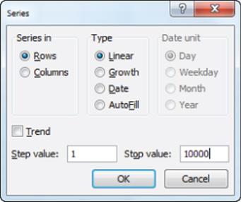
Figure 21-4: Land's End data table

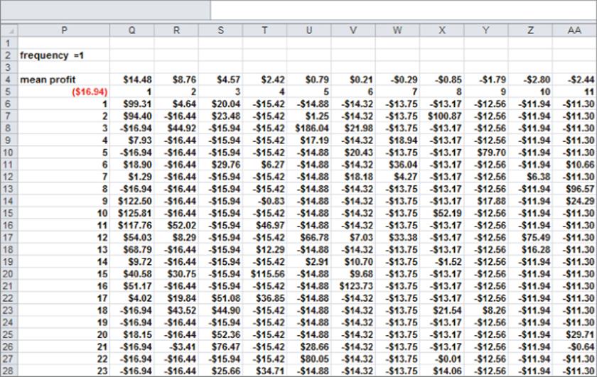
You can now estimate that a customer who purchased from the last received catalog is worth $14.48; a customer who last purchased two catalogs ago is worth $8.76; and so on. Customers who last ordered seven or more catalogs ago have negative value, so you should stop mailing to these customers.

Using Monte Carlo Simulation to Predict Success of a Marketing Initiative

When a company is considering a marketing decision, they never know with 100 percent certainty that their decision will make the company better off. If a company repeatedly chooses marketing decisions that have much more than a 50 percent probability of making the company better off, then in the long run the company will succeed as result of marketing decisions. You can use Monte Carlo simulation to evaluate the probability that a marketing decision will improve a company's bottom line. In this section you will learn how to do this by analyzing whether a pizza parlor will benefit from a Groupon offer.

Carrie has just been fired from the CIA and has purchased a suburban Virginia pizza parlor. She is trying to determine whether she should offer the local residents a Groupon offer. As discussed in Chapter 19, “Calculating Lifetime Customer Value,” Groupon offers customers pizza for less than cost. The restaurant hopes to recoup the loss on the pizzas sold with a Groupon offer via the customer value of new customers who become return customers. To be specific, the terms of the Groupon offer follow:

· Customers are offered two pizzas (usually sold for $26) for $10.

· Carrie keeps half of the revenue ($5).

· Carrie's profit margin is 50 percent.

In deciding whether to use Groupon, Carrie faces many sources of uncertainty:

· Fraction of customers who take the offer who are new customers

· Fraction of people who spend more than the deal size ($26)

· For customers who spend more than $26, the amount spent in excess of $26

· Fraction of new customers who return

· Annual profit generated by new customers who return

· Retention rate for new customers

To help Carrie determine the range of outcomes that will result from the Groupon offer, you can use the Monte Carlo simulation to model these sources of uncertainty and in doing so, estimate the chances that the Groupon offer will increase profitability. The key to the analysis is using the customer value concepts of Chapter 19 and the Monte Carlo simulation to estimate the probability that the benefit the pizza parlor gains from new customers will outweigh the lost profit on pizzas sold to customers who redeem the Groupon offer.

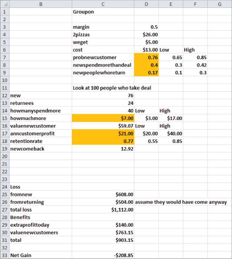
To simplify modeling, assume each of the six uncertain quantities is equally likely to assume any value between a low value and a high value. The low and high values for these quantities are shown in Figure 21.5.

Figure 21-5: Analysis of Groupon for Carrie's Pizza

When trying to determine these values, the marketing analyst can use historical information to establish upper and lower bounds. In his 2011 paper “What Makes Groupon Promotions Profitable for Businesses?”, Utpal Dhoakia surveyed 324 businesses that used Groupon and obtained estimates for some of the previously listed quantities:

· 75 percent of people taking the deal are new customers.

· 36 percent of all deal takers spent more than the deal size.

· 20 percent of new customers returned later.

Based on this information and on past Groupon offers, Carrie believes the following:

· Between 65 percent and 85 percent of customers taking the deal will be new customers.

· Between 30 percent and 42 percent of customers will spend an amount in excess of $26.

· Those who spend in excess of $26 will spend on average between $3 and $17 beyond $26.

· Between 10 percent and 30 percent of new customers will return.

· Average annual profit generated by a new customer is between $20 and $40.

· Average annual retention rate for new customers generated by Groupon is between 55 percent and 85 percent.

You can use the Excel RANDBETWEEN function to ensure that an uncertain quantity (often called a random variable) is equally likely to lie between a lower limit L and an upper limit U. For integers, entering the formula RANDBETWEEN(L,U) in a cell makes it equally likely that any integer between L and U inclusive will be entered in the cell. For example, entering the formula =RANDBETWEEN(65,85) in a cell ensures that it is equally likely that any of 65, 66, …, 84, or 85 is entered in the cell.

Complete the following steps (see the file Groupon.xlsx) to model the range of outcomes that will ensue if Carrie introduces a Groupon offer:

1. In D3:D5 enter Carrie's profit margin, the price of two pizzas without Groupon, and what Carrie receives from Groupon for two pizzas.

2. In D6 compute the cost of producing two pizzas with the formula =(1-margin)*_2pizzas.

3. In cell D7 enter the fraction of Groupon offer takers who are new customers with the formula =RANDBETWEEN(100*E7,100*F7)/100. This is equally likely to enter a .65, .66, …, .84, .85 in cell D7.

4. In cell D8 generate the fraction of new customers who spend more than $26 with the formula =RANDBETWEEN(100*E8,100*F8)/100.

5. Copy this formula from cell D8 to D9 to generate the fraction of new Groupon customers who return.

6. Assume without loss of generality that 100 customers take the Groupon offer and you generate the random net gain (or loss) in profit from these 100 offer takers. Include gains or losses today and gains from added new customers.

7. In cell C12 compute the number of your 100 offer takers who will be new customers with the formula =100*probnewcustomer.

8. In cell C13 compute the number of offer takers who are returnees with the formula =100*(1-probnewcustomer).

9. In cell C14 compute the number of offer takers who spend more than the deal with the formula =100*newspendmorethandeal.

10. In cell C15 determine the average amount spent in excess of $26 by those spending more than $26 with the formula =RANDBETWEEN(D15,E15). Copy this formula to C17 to determine the average level of annual customer profit for new customers created by the Groupon offer.

11. In the worksheet basic model, attach your Customer Value template, as discussed in Chapter 19. Then in C16 use the formula ='basic model'!E5*C17 to compute the lifetime value of a customer based on mid-year cash flows.

12. In cell C18 compute the average retention rate for new customers with the formula =RANDBETWEEN(100*D18,100*E18)/100.

13. In cell C19 compute the number of the 100 offer takers who are returning new customers with the formula =C12*newpeoplewhoreturn.

In the range C25:C33 you can compute your gain or loss from the 100 offer takers:

1. To begin in cell C25, use the formula =(cost-weget)*C12 to compute your loss today from the new customers among the offer takers as $8 * number of new customers.

2. To simplify your work assume all offer takers who were previous customers would have shown up anyway. Because each of these returning customers would have paid $26, you lose $26 – $5 = $21 on each of these customers.

3. Then in cell C26 use the formula =C13*(_2pizzas-weget) to compute your loss on these customers.

4. In cell C27 the formula =SUM(C25:C26) computes your total loss today on the 100 people who took the Groupon offer.

5. In C29 with the formula =margin*C15*C14, compute the extra profit earned today by multiplying your 50 percent profit margin by the amount in excess of $26 spent today by offer takers.

6. In C30 use the formula =C19*C16 to compute the value of the new customers by multiplying the number of returning new customers times the average value for each new customer.

7. In cell C31 use the formula =C29+C30 to compute the total benefits created by the Groupon offer.

8. In cell C33 use the formula =C31-C27 to compute the total benefits less today's losses.

Using a One-Way Data Table to Simulate the Groupon Deal

You can now use Monte Carlo simulation (via a one-way data table) to “play out” the spreadsheet 10,000 times. Then tabulate your average gain per offer taker and the probability that the Groupon offer will increase Carrie's long-term bottom line.

1. Use FILL SERIES (from the Home tab) to enter the iteration numbers (1, 2, …, 10,000) in the range I9:I10008.

2. Use a one-way data table to “trick” Excel into replaying your spreadsheet 10,000 times. Recalculate your total gain on the 100 offer takers, so enter the total gain in cell J8 with the formula =C33.

3. Select the data table range (I8:J10008), and from the Data tab, choose What-If Analysis and select Data Table… In a one-way data table, there is no row input cell, so all you need to do is choose any blank cell (such as N7) as the column input cell. Then Excel places 1, 2, …, 10,000 in N7 and each time recalculates Carrie's net gain. During each recalculation each RANDBETWEEN function recalculates, so you play out the modeled uncertainty 10,000 times. The resulting simulated profits are shown in the range J9:J10008 of Figure 21.6.

4. In cell K3 compute the average profit over your 10,000 iterations earned from the 100 deal takers with the formula =AVERAGE(J9:J10008). You find an average gain of $144.11, which indicates that on average the Groupon deal can improve Carrie's bottom line.

5. In cell K4 compute the probability that the deal increases profits with the formula =COUNTIF(J9:J10008,">0")/10000. There is a 53.8 percent chance the deal yields a favorable result.

Figure 21-6: Simulation results for Carrie's Pizza

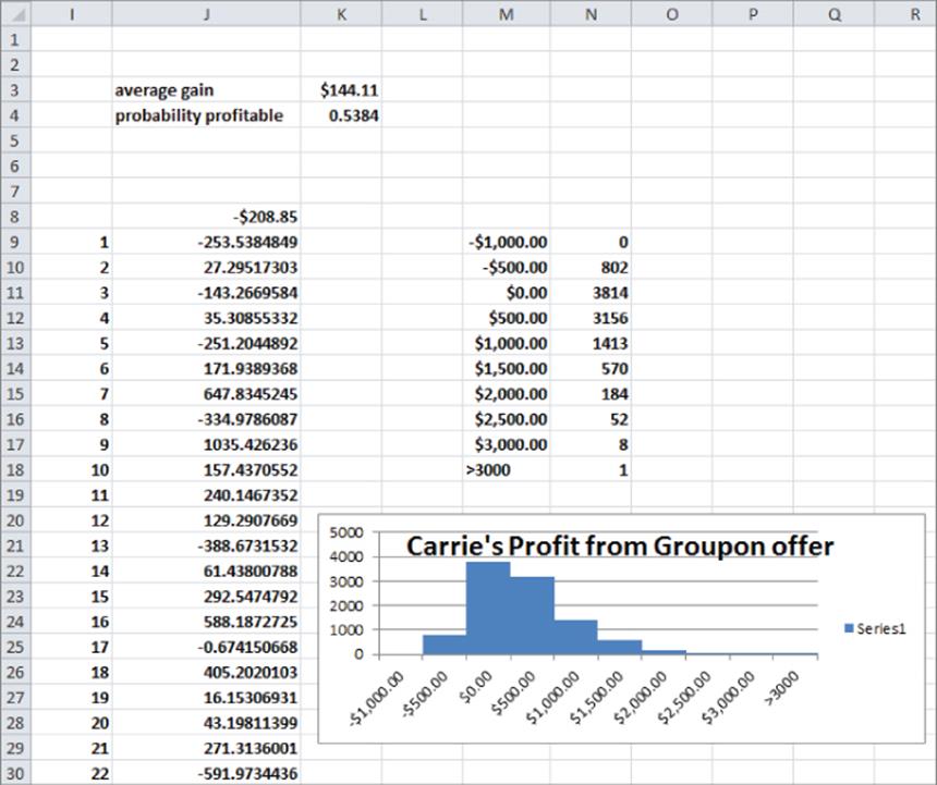
This finding indicates that the deal is of marginal value to the pizza parlor. From cell K3, you find that the average profit per customer equals $144.11. This again indicates that on average, the Groupon deal does just a little better than breaking even.

Using a Histogram to Summarize the Simulation Results

As the Chinese say, “A picture is worth a thousand words.” With this in mind use a bar graph or histogram to summarize your simulation results. To create a bar graph of your simulation results, proceed as follows:

1. Enter the boundaries of bin ranges (–$1000, –$500, …, $3000) in M9:M17. Append a label >3000 for all iterations in which profit is more than $3000.

2. Select the range N9:N18 and array enter by selecting Ctrl+Shift+Enter (see Chapter 2, “Using Excel Charts to Summarize Marketing Data”) the formula =FREQUENCY(J9:J10008,M9:M17). In N9 this computes the number of iterations in which profit is <=$1000; in N10 this array formula computes the number of iterations in which profit is >–$1000 and <=–$500 (802); in N18 this array formula computes the number of iterations (1) in which profit is >$3000.

A column graph summarizing these results is shown in Figure 21.6.

Summary

You can use the Excel data table feature combined with Excel's RAND() and RANDBETWEEN functions to simulate uncertainty in situations in which customer value involves uncertain quantities (random variables).

· If an uncertain event has a probability x of occurring, then the event occurs if a value of RAND() is less than or equal to x.

· If an uncertain quantity (such as annual retention rate) is normally distributed with a given mean and sigma, then the function =NORMINV(RAND(),mean,standard dev) generates a normal random variable with the given mean and sigma.

· If an uncertain quantity (such as annual profit generated by a customer) is equally likely to be between two integers L and U, then it can be modeled with the function RANDBETWEEN(L,U).

Exercises

1. Suppose each customer purchase of a product generates $10 in profit. Each month a customer either buys 0 or 1 unit of the product. If a customer bought last month, there is a 0.5 chance she will buy next month. If she last bought two months ago, there is a 0.2 chance she will buy next month. If she last bought three months ago, there is a 0.1 chance that she will buy next month. If a customer has not bought for four months, there is no chance she will ever buy in the future. Determine the value of a customer who last purchased the product last month, two months ago or three months ago. Assume profits are discounted at 1 percent per month.

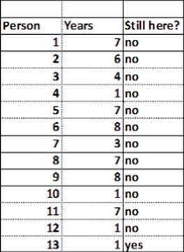
2. You own a business magazine CY. At the beginning of year 1, you have 300,000 subscribers and 700,000 nonsubscribers who are considered possible subscribers in the future. Determine whether it is a good idea to give prospective subscribers their first year subscription for free. The fileCustomerdata.xlsx gives for a random sample of subscribers the number of years they subscribed. A sample of the data is shown in Figure 21.7. For example, Person 2 subscribed for six years before canceling, and Person 13 has subscribed for one year and is still a subscriber. To begin, use this data to estimate the annual retention rate, assuming that retention rate does not depend on how long a person has subscribed.

Figure 21-7: Retention data for CY magazine

(a) Currently the annual subscription fee is $55 and you make $50 annual profit per subscriber (based on beginning of year subscribers.) You discount cash flows at 10 percent per year. At present 5 percent of the nonsubscribers at the beginning of a year become subscribers at the beginning of the next year. At the beginning of each year, 20,000 new nonsubscribers enter the market. After a person stops being a subscriber, assume he will never subscribe again. Determine the value of the status quo. Use 20 years and assume at the beginning of year 21 each current subscriber is credited with a salvage value based on the Customer Value template.

(b) CY is considering giving new subscribers their first year for free. You are not sure how this will increase the fraction of nonsubscribers you get each year above the current level of 5 percent, but you estimate the new recruitment percentage will be normally distributed with a mean of 6 percent and a standard deviation of 1 percent. Assume that the recruitment rate of new subscribers will be the same each year. Also assume that all cash flows occur at the beginning of a year and there is no customer acquisition cost. Use the output from 10,000 iterations of a Monte Carlo simulation to determine whether you should give the new subscribers the first year for free.

3. You work for OJ's Orange Juice. Currently there are 10 million customers, and each week a customer buys 1 gallon of orange juice from OJ or a competitor. The current profit margin is $2 per gallon. Last week six million customers bought from you, and four million bought from the competition.

The file OJdata.xlsx gives the purchase history for a year for several customers. For example, in week three, Person 5 did not buy from you (0 = bought from competition, 1 = bought from you). The data is scrambled so you need to manipulate it. From this data you should figure out the chance customers will buy from you next week if they bought from you last week and the chance customers will buy from you next week if they bought from a competitor last week. Solve the following situations:

(a) Evaluate the profitability of the status quo (for 52 weeks including the current week). No need for discounting!

(b) OJ Orange Juice is considering a quality improvement. This improvement will reduce per-gallon profitability by 30 cents. This will increase customer loyalty, but you are not sure by how much. Assume it is equally likely that the customer retention rate will increase by between 0 percent and 10 percent. Use 10,000 iterations of a Monte Carlo simulation to determine whether OJ should make the quality improvement. Use a single RANDBETWEEN random variable to model the average improvement in customer loyalty created by the quality improvement.

4. GM wants to determine whether to give a $1,000 incentive this year to buyers of Chevy Malibus. Here is relevant information for the base case:

· Year 1 price: $20,000

· Year 1 cost: $16,000

· Each year 30 percent of the market buys a Malibu or a car from the competition.

· Seventy percent of people who last bought a Malibu will make their next purchase a Malibu.

· Twenty-five percent of people who last bought a car from the competitor will make their next purchase a Malibu.

· Inflation is 5 percent per year (on costs and price).

· Currently 50 percent of the market is loyal to Malibu, and 50 percent is loyal to the competition.

· Profits are accrued at the beginning of the year and are discounted at 10 percent per year.

GM is considering giving a $1,000 incentive to any year 1 purchaser. The only change in the base numbers are as follows:

· The percentage of the market buying a Malibu or a car from the competition in year 1 will increase by between 2 percent and 10 percent.

· The fraction of loyal people who will make their next purchase in year 1 a Malibu will increase by between 5 percent and 15 percent.

· The fraction of non-loyal people who will make their next purchase in year 1 a Malibu will increase by between 6 percent and 13 percent.

Answer the following questions:

(a) Assuming end of year cash flows and a 30-year planning horizon, should Chevy give the $1,000 incentive? To answer this question, use the output from 10,000 iterations of a Monte Carlo simulation.

(b) Suppose the discount rate decreased to 7 percent. Would your decision change? Explain your answer without any calculations.

(c) Suppose the year 1 price increased to $22,000. Would your decision change? Explain your answer without any calculations.

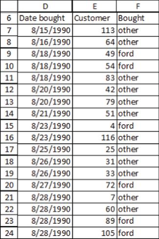
5. The local Ford dealer wants to determine whether to give all purchasers of new cars free oil changes. The Forddata.xlsx contains information on loyalty of car purchasers. A sample of this data is shown in Figure 21.8. For example, the data in row 7 indicates that customer number 113 bought a non-Ford on 8/15/1990.

Use this data to determine the current chance that a Ford purchaser will next buy a Ford and the current chance a purchaser of another type of car will next buy a Ford. You have the following information:

Figure 21-8: Purchase data for Ford dealer

· The length of time a person keeps a new car is equally likely to be between 700 and 2,000 days.

· Ford makes $2,000 on the purchase of a new car.

· Without free oil changes Ford earns $350 profit per year from servicing a car.

· Currently customers pay $100 per year for oil changes, which cost Ford $60 to perform. Assume all Ford purchasers always have their oil changed at the dealer.

· All purchase and service profits are booked at the time the car is purchased, and profits are discounted at 10 percent per year.

· If you give free oil changes, loyalty percentages and switch percentages will improve by an unknown amount, equally likely to be between 2 percent and 15 percent.

Suppose a customer has bought a car from a competitor today. Determine the 20-year value of this customer to Ford without the free oil changes. What is the chance that the free oil changes increase the value of this customer?