Marketing Analytics: Data-Driven Techniques with Microsoft Excel (2014)

Part V. Customer Value

Chapter 22. Allocating Marketing Resources between Customer Acquisition and Retention

In the discussion of customer value so far, the retention rate has been assumed as a given. In reality, a firm can increase its retention rate by spending more money on customer retention. For example, Verizon could put more customer service representatives in stores to provide customers with better technical support and reduce store waiting times. This would cost Verizon money, but would likely increase its customer retention rate. Verizon could also increase the number of new customers by spending more money on customer acquisition. Robert Blattberg and John Deighton (Manage Marketing by the Customer Equity Test, Harvard Business Review, 1996, Vol. 74, No. 4, pp. 136–144) were the first to realize that companies could optimize profits by adjusting expenditures on retention and acquisition. This chapter explains and extends their model to show how companies can determine if they are spending too much (or too little) on customer retention and customer acquisition.

Modeling the Relationship between Spending and Customer Acquisition and Retention

Companies need to determine how much money to spend acquiring new customers and how much money to spend retaining current customers. The first step in optimizing spending is to develop a functional relationship that explains how increased spending leads to more customer retention or acquisition. Following Blattberg and Deighton (1996), assume the following equations are true:

1

2

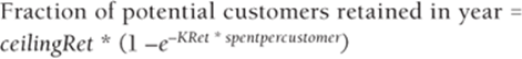
The ceilingRet is the fraction of current customers you would retain during a year if you spent a saturation level of money on retention. Note that as spentpercustomer grows large, the fraction of potential customers retained in a year approaches ceilingRet. Given an estimate of ceilingRet and current retentionrate (based on current spending) you can use Equation 1 to solve for kRet (see Exercise 3.) You can find that the following is true:

3

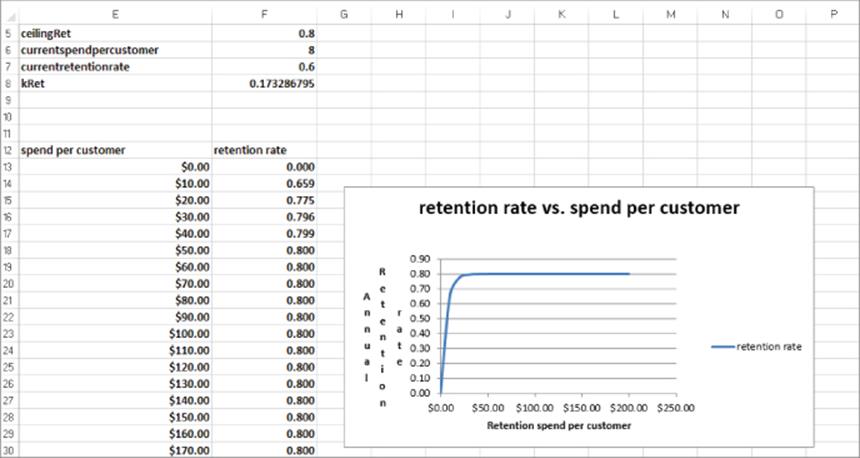
Given the currentretentionrate, ceilingRet, and currentspendpercustomer, you can use the file Retentiontemplate.xlsx (see Figure 22.1) to calculate kRet. For example, if you are given that current spending of $40 per customer yields a retention rate of 60 percent and a saturation level of spending yields an 80 percent retention rate, then kRet = 0.034657. Figure 22.1 shows how additional spending on retention yields diminishing returns in improving the retention rate. In essence the value of kRet governs the speed at which the retention rate approaches its ceiling. The larger the value of kRet, the faster the retention rate approaches its ceiling value.

Figure 22-1: Retention rate as a function of retention spend per customer

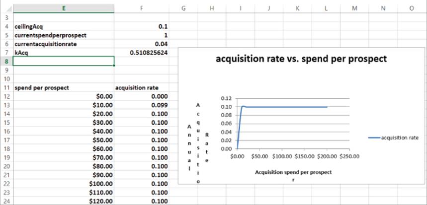
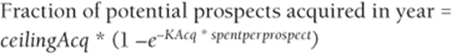
The ceilingAcq is a fraction of the potential prospects you would attract in a year if you spent a saturation level of money on customer acquisition. Note that as spendperprospect grows large, the annual fraction of prospects acquired in a year approaches the ceiling. Given an estimate for the ceiling and current acquisition rate (based on current spending) you can use Equation 2 to solve for the value of k in Equation 4, as shown in the acquisition worksheet of the Retentiontemplate.xlsx file:

4

For example, suppose that spending $40 a year per prospective customer yielded an annual acquisition rate of 5 percent of potential customers (shown in Figure 22.2). Also suppose that spending a saturation level of money on acquisition raises the acquisition rate to 10 percent. Then k = 0.01732868.

Figure 22-2: Acquisition rate as a function of acquisition spend per prospect

After you have fit Equations 1 and 2, you can use Solver to optimize acquisition and retention spending over a time horizon of arbitrary length.

Basic Model for Optimizing Retention and Acquisition Spending

In this section you will learn how the Excel Solver can be used to determine an optimal allocation of marketing expenditures to activities related to acquiring and retaining customers.

Carrie's Pizza wants to determine the level of acquisition and retention spending that maximizes net present value (NPV) of profits over a 20-year planning horizon. The following summarizes relevant information:

· Carrie's Pizza currently has 500 customers and its potential market size is 10,000.

· Carrie's earns $50 profit per year (exclusive of acquisition and retention costs) per customer.

· Carrie's Pizza currently spends $1.00 each year per prospect and attracts 4 percent of all prospects. It estimates that if a lot of money were spent on acquisition during a year, it would acquire 10 percent of all prospects.

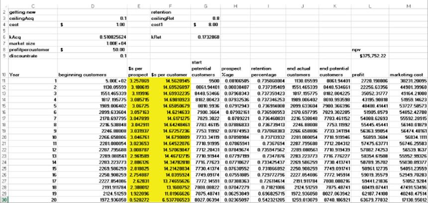
· Carrie's Pizza currently spends $8 per year on each customer in customer retention efforts and retains 60 percent of all customers. Carrie's Pizza believes that if it spends a lot on customer retention, it will retain 80 percent of all customers. Assuming a 10 percent annual discount rate, the initial solution to this problem is in the worksheet original of the customerretentionoriginal.xls workbook (see Figure 22.3).

· From cell F7 of the worksheet acquisition (see Figure 22.2) in the workbook Retentiontemplate.xlsx you find that kAcq = 0.510825824, and from cell F8 of the worksheet retention (see Figure 22.1) in the workbook Retentiontemplate.xlsx you find that kRet = 0.173287. Once you find this, you can enter trial values for years 1–20 of acquisition per prospect and retention spending per customer in E11:F30. This will track Carrie's Pizza's number of customers each year and the associated profits and costs.

Figure 22-3: Basic model for optimizing retention and acquisition spending

Begin with any trial values for annual expenditures on acquisition and retention spending entered in the range E11:F30. You can then use Solver to determine the annual spending that maximizes Carrie's Pizza's 20-year NPV. No matter what the starting point, the Solver will find the values of annual spending on acquisition and retention that maximize Carrie's 20-year NPV. Proceed as follows:

1. Enter the beginning customers in D11, enter trial acquisition spending per prospect in E11:E30, and enter trial retention spending per customer in F11:F30.

2. Compute the beginning potential customers in G11 with formula =market_size-D11.

3. Copy the formula =ceiling*(1-EXP(-kAcq*E11)) from H11 to H12:H30 to compute the percentage of prospects acquired during each year.

4. Copy the formula =ceilingRet*(1-EXP(-Ret_*F11)) from I11 to I12:I30 to compute the fraction of all customers retained during each year.

5. Copy the formula =I11*D11+H11*G11 from J11to J12:J30 to add together new and retained customers to compute the number of customers at the end of each year.

6. Copy the formula =market_size-J11 from K11 to K12:K30 to compute the number of prospects at the end of each year.

7. Copy the formula =0.5*profitpercustomer*(D11+J11)-E11*G11-F11*D11 from L11 to L12:L30 to compute the profit for each year. Note that you average beginning and ending customers to get a more accurate estimate of the average number of customers present during the period.

8. Copy the formula =E11*G11-F11*D11 from M11 to M12:M30 to compute the total marketing cost during each year.

9. Copy the formula =J11 from D12 to D13:D30 to ensure that each month's beginning customers equal the previous month's ending customers.

10. Assuming end-of-year cash flows, compute total NPV of profits in cell L9 with the formula =NPV(D9,L11:L30).

11. Use the Solver settings shown in Figure 22.4 to choose the annual levels of retention and acquisition spending that maximize the 20-year NPV end-of-year profits.

Figure 22-4: Solver settings for basic model

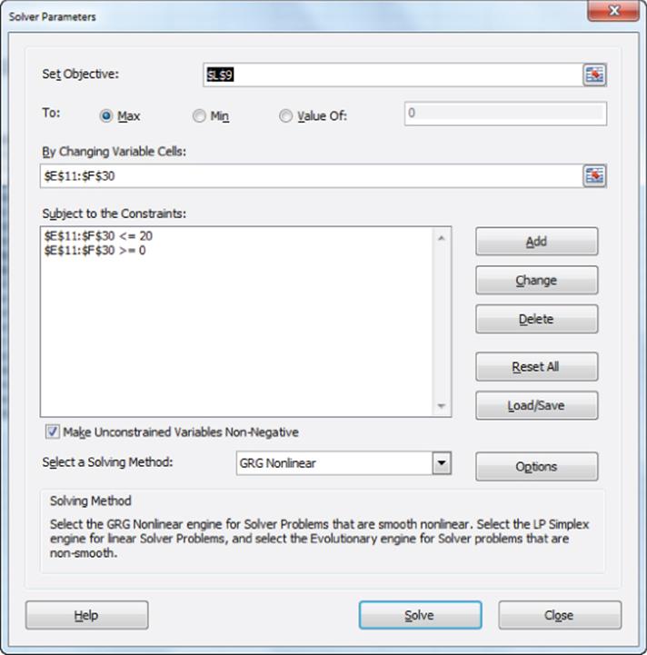
You bounded spending on acquisition and retention per person during each year by $20. (This bound was unnecessary, however, because the optimization did not recommend spending that much money). Note that if during any month the per capita expenditure recommended by Solver were $20, you would have increased the upper bound.

Solver found a maximum NPV of approximately $376,000. During most years you spend approximately $3 per prospect on acquisition and $14 per customer on retention. Given the cost structure you try during most years, you retain 73 percent of the customers and acquire 8 percent of the prospects.

An Improvement in the Basic Model

The basic model discussed in the last section has a small flaw: in the last few years the spending drops. This is because a customer acquired in, say, year 19, generates only one year of profit in the model. Because a customer acquired in year 19 yields little profit, you do not spend much to get her. If the model is valid, the spending on acquisition or retention should not sharply decrease near the end of the planning horizon. To remedy this problem you need to give an ending credit or salvage value for a customer left at the end of the planning horizon. To accurately determine the value of a customer, follow these steps using the customerretentionsalvage.xls workbook shown in Figure 22.5.

1. To begin, copy the formulas from the original worksheet down to row C34 (see Figure 22.5) and add in cell I8 as a trial value for the value of a single customer who has just been acquired.

2. Using a Solver constraint, force the customer value for the second set of formulas (listed in cell I40) to equal I8.

3. Add one more initial customer to cell D41 and start with 501 customers.

4. In both parts of the spreadsheet, assign each ending customer a salvage value by adding the term J63*I40 to cell L63 and adding the term J31*I8 to cell L31.

5. In cell L2 compute the difference between the two situations with the formula =L42-L10 (see Figure 22.6). Also constrain the spending levels in rows 44–63 to equal the spending levels in rows 12–31. The Solver window is shown in Figure 22.7.

Figure 22-5: Model with customer salvage value

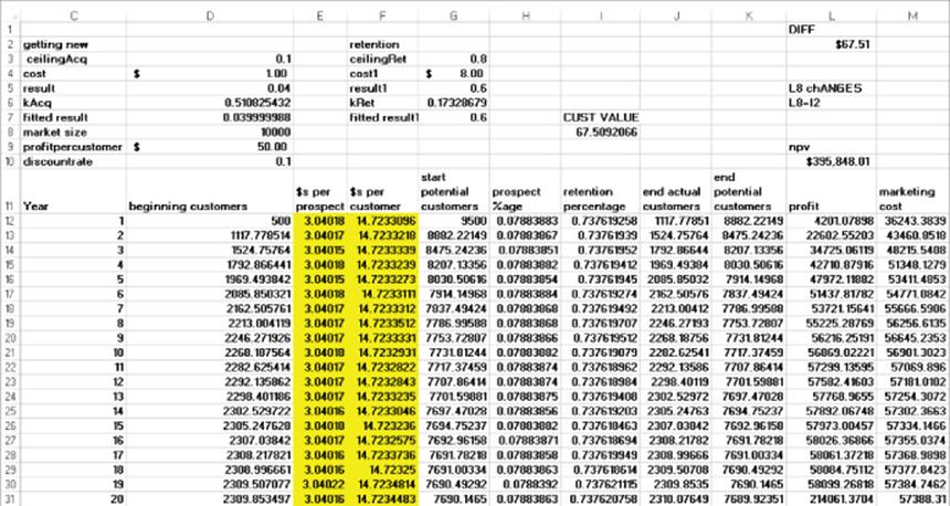
Figure 22-6: Customer value for salvage value model

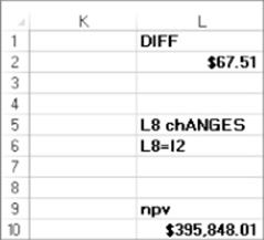
Figure 22-7: Solver settings for salvage value model

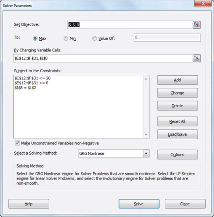
The Solver window changes in two ways:

· The value of an individual customer (I8) is added as a changing cell.

· A constraint that L2=I8 is added. This constraint ensures that the customer value in cell I8 indeed equals the amount you gain by adding one more customer. This consistency constraint ensures that Solver will make the value in cell I8 equal the true value of a customer. Because you are now properly accounting for the ending value of a customer, the model now ensures you do not reduce spending near the end of the planning horizon.

Running Solver yields the spending levels shown in Figure 22.5 and the individual customer value shown in Figure 22.6. The optimal spending for the acquisition is approximately $3.04 per customer every year, and approximately $14.71 per customer is spent each year on retention. The value of a customer is $67.51.

Summary

In this chapter you have learned the following:

· To determine the profit maximizing expenditures on customer acquisition and retention, assume the following equations are true:

(1)

(2)

· Given assumptions on the maximum attainable retention (ceilingRet) and acquisition (ceilingAcq) rates and the current spending on retention and acquisition, you can use Equations 3 and 4 or the workbook Retentiontemplate.xlsx to solve for kRet and kAcq.

· The Solver can determine the annual levels of per capita retention and acquisition spending that maximizes the NPV of profits.

· If desired you may account for the salvage value of a customer to ensure that spending levels remain unchanged throughout the planning horizon.

Exercises

1. Verizon is trying to determine the value of a cell phone subscriber in Bloomington, Indiana, and the optimal levels of acquisition and retention spending. Currently Verizon has 20,000 customers and 30,000 potential customers. You are given the following information:

· Profits are discounted at 10 percent per year.

· Annual profit per customer is $400.

· Currently Verizon is spending $12 per prospect on acquisition and capturing 4 percent annually of prospective customers.

· Currently Verizon is spending $30 per customer on customer retention and has a retention rate of 75 percent.

· Verizon believes that with a saturation level of spending, the annual acquisition rate would increase to 10 percent and the annual retention rate would increase to 85 percent.

(a) Determine the value of a customer and the profit maximizing annual level of acquisition and retention spending.

(b) Use SolverTable to determine how the optimal level of retention and acquisition spending in Exercise 1 varies with an increase in annual profit.

2. Verify Equation 3.