Marketing Analytics: Data-Driven Techniques with Microsoft Excel (2014)

Part VI. Market Segmentation

Chapter 23: Cluster Analysis

Chapter 24: Collaborative Filtering

Chapter 25: Using Classification Trees for Segmentation

Chapter 23. Cluster Analysis

Often the marketer needs to categorize objects into groups (or clusters) so that the objects in each group are similar, and the objects in each group are substantially different from the objects in the other groups. Here are some examples:

· When Procter & Gamble test markets a new cosmetic, it may want to group U.S. cities into groups that are similar on demographic attributes such as percentage of Asians, percentage of Blacks, percentage of Hispanics, median age, unemployment rate, and median income level.

· An MBA chairperson naturally wants to know the segment of the MBA market in which her program belongs. Therefore, she might want to cluster MBA programs based on program size, percentage of international students, GMAT scores, and post-graduation salaries.

· A marketing analyst at Coca-Cola wants to segment the soft drink market based on consumer preferences for price sensitivity, preference of diet versus regular soda, and preference of Coke versus Pepsi.

· Microsoft might cluster its corporate customers based on the price a given customer is willing to pay for a product. For example, there might be a cluster of construction companies that are willing to pay a lot for Microsoft Project but not so much for Power Point.

· Eli Lilly might cluster doctors based on the number of prescriptions for each Lilly drug they write annually. Then the sales force could be organized around these clusters of physicians: a GP cluster, a mental health cluster, and so on.

This chapter uses the first and third examples to learn how the Evolutionary version of the Excel Solver makes it easy to perform a cluster analysis. For example, in the U.S. city illustration, you can find that every U.S. city is similar to Memphis, Omaha, Los Angeles, or San Francisco. You can also find, for example, that the cities in the Memphis cluster are dissimilar to the cities in the other clusters.

Clustering U.S. Cities

To illustrate the mechanics of cluster analysis, suppose you want to “cluster” 49 of America's largest cities (see the cluster.xls file for the data and analysis, as well as Figure 23.1). For each city you have the following demographic data that will be used as the basis of your cluster analysis:

· Percentage Black

· Percentage Hispanic

· Percentage Asian

· Median age

· Unemployment rate

· Per capita income

Figure 23-1: Data for clustering U.S. cities

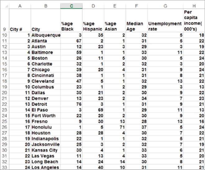
For example, Atlanta's demographic information is as follows: Atlanta is 67 percent Black, 2 percent Hispanic, 1 percent Asian, has a median age of 31, a 5 percent unemployment rate, and a per capita income of $22,000.

For now assume your goal is to group the cities into four clusters that are demographically similar. Later you can address the issue of why you used four clusters. The basic idea used to identify the clusters is to choose a city to “anchor,” or “center,” each cluster. You assign each city to the “nearest” cluster center. Your target cell is then to minimize the sum of the squared distances from each city to the closest cluster anchor.

Standardizing the Attributes

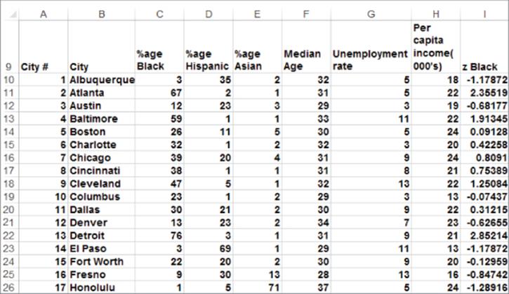
In the example, if you cluster using the attribute levels referred to in Figure 23.1, the percentage of Blacks and Hispanics in each city will drive the clusters because these values are more spread out than the other demographic attributes. To remedy this problem you can standardize each demographic attribute by subtracting off the attribute's mean and dividing by the attribute's standard deviation. For example, the average city has 24.34 percent Blacks with a standard deviation of 18.11 percent. This implies that after standardizing the percentage of Blacks, Atlanta has 2.35 standard deviations more Blacks (on a percentage basis) than a typical city. Working with standardized values for each attribute ensures that your analysis is unit-free and each attribute has the same effect on your cluster selection. Of course you may give a larger weight to any attribute.

Choosing Your Clusters

You can use the Solver to identify a given number of clusters. The key in doing so is to ensure that the cities in each cluster are demographically similar and cities in different clusters are demographically different. Using few clusters enables the marketing analyst to reduce the 49 U.S. cities into a few (in your case four) easily interpreted market segments. To determine the four clusters, as shown in Figure 23.2, begin by computing the mean and standard deviation for Black percentage in C1:G2.

1. Compute the Black mean percentage in C1 with the formula =AVERAGE(C10:C58).

2. In C2 compute the standard deviation of the Black percentages with the formula =STDEV(C10:C58).

3. Copy these formulas to D1:G2 to compute the mean and standard deviation for each attribute.

4. In cell I10 (see Figure 23.3) compute the standardized percentage of Blacks in Albuquerque (often called a z-score) with the formula =STANDARDIZE(C10,C$1,C$2). This formula is equivalent, of course, to . The reader can verify (see Exercise 6) that for each demographic attribute the z-scores have a mean of 0 and a standard deviation of 1.

5. Copy this formula from I10 to N58 to compute z-scores for all cities and attributes.

Figure 23-2: Means and standard deviations for U.S. cities

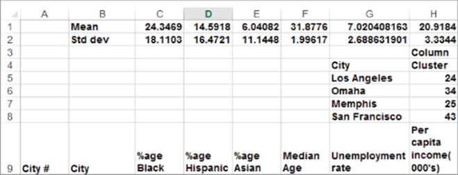
Figure 23-3: Standardized demographic attributes

How Solver Finds the Optimal Clusters

To determine n clusters (in this case n = 4) you define a changing cell for each cluster to be a city that “anchors” the cluster. For example, if Memphis is a cluster anchor, each city in the Memphis cluster should be similar to Memphis demographically, and all cities not in the Memphis cluster should be different demographically from Memphis. You can arbitrarily pick four cluster anchors, and for each city in the data set, you can determine the squared distance (using z-scores) of each city from each of the four cluster anchors. Then you assign each city the squared distance to the closest anchor and have your Solver target cell equal the sum of these squared distances.

To illustrate how this approach can find optimal clusters, suppose you ask a set of moviegoers who have seen both Fight Club and Sea Biscuit to rate these movies on a 0–5 scale. The ratings of 40 people for these movies are shown in Figure 23.4 (see file Clustermotivation.xlsx).

Figure 23-4: Movie ratings

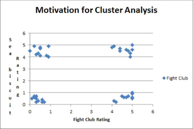
Looking at the chart it is clear that the preference of each moviegoer falls into one of four categories:

· Group 1: People who dislike Fight Club and Sea Biscuit (lower-left corner)

· Group 2: People who like both movies (upper-right corner)

· Group 3: People who like Fight Club and dislike Sea Biscuit (aka people with no taste in the lower-right corner)

· Group 4: People who like Sea Biscuit and hate Fight Club (aka smart people in the upper-left corner)

Suppose you take this data and set up four changing cells, with each changing cell or anchor allowed to represent the ratings of any person (refer to Figure 23.4). Let each point's contribution to the target cell be the squared distance to the closest anchor. Then choose one anchor from each group to minimize the target cell. This ensures each point is “close” to an anchor. If, for example, Solver considers two anchors from Group 1, one from Group 3, and one from Group 4, this cannot be optimal because swapping out one Group 1 anchor for a Group 2 anchor would lessen the target cell contribution from the 10 Group 2 points, while hardly changing the target cell contribution from the Group 1 points. Therefore you must only have one anchor for each group. You can now implement this approach for the Cities example.

Figure 23.5 Look up z-scores for cluster anchors

Setting Up the Solver Model for Cluster Analysis

For the Solver to determine four suitable anchors you must pick a trial set of anchors and figure out the squared distance of each city from the closest anchor. Then Solver can pick the set of four anchors that minimizes the sum of the squared distances of each city from its closest anchor.

To begin, set up a way to “look up” the z-scores for candidate cluster centers:

1. In H5:H8 enter “trial values” for cluster anchors. Each of these values can be any integer between 1 and 49. For simplicity you can let the four trial anchors be cities 1–4.

2. After naming A9:N58 as the range lookup in G5, look up the name of the first cluster anchor with the formula =VLOOKUP(H5,Lookup,2).

3. Copy this formula to G6:G8 to identify the name of each cluster center candidate.

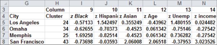
4. In I5:N8 identify the z-scores for each cluster anchor candidate by copying from I5 to I5:N8 the formula =VLOOKUP($H5,Lookup,I$3).

You can now compute the squared distance from each city to each cluster candidate (see Figure 23.6.)

1. To compute the distance from city 1 (Albuquerque) to cluster candidate anchor 1, enter in O10 the formula =SUMXMY2($I$5:$N$5,$I10:$N10). This cool Excel function computes the following:

(I5-I10)²+(J5-J10)²+(K5-K10)²+(L5-L10)²+(M5-M10)²+(N5-N10)²

2. To compute the squared distance of Albuquerque from the second cluster anchor, change each 5 in O10 to a 6. Similarly, in Q10 change each 5 to a 7. Finally, in R10 we change each 5 to an 8.

3. Copy from O10:R10 to O11:R58 to compute the squared distance of each city from each cluster anchor.

4. In S10:S58 compute the distance from each city to the “closest” cluster anchor by entering the formula =MIN(O10:R10) in cell S10 and copying it to the cell range S10:S59.

5. In S8 compute the sum of squared distances of all cities from their cluster anchor with the formula =SUM(S10:S58).

6. In T10:T58 compute the cluster to which each city is assigned by entering in T10 the formula =MATCH(S10,O10:R10,0) and copying this formula to T11:T58. This formula identifies which element in columns O:R gives the smallest squared distance to the city.

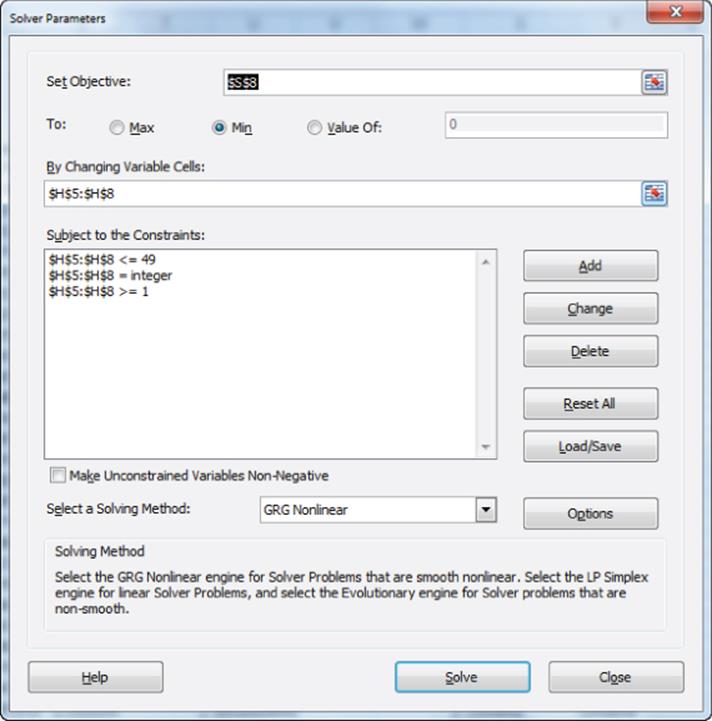
7. Use the Solver window, as shown in Figure 23.7, to find the optimal cluster anchors for the four clusters.

NOTE

Cell S8 (sum of squared distances) is minimized in the example. The cluster anchors (H5:H8) are the changing cells. They must be integers between 1 and 49.

8. Choose the Evolutionary Solver. Select Options from the Solver window, navigate to the Evolutionary tab, and increase the Mutation rate to 0.5. This setting of the Mutation rate usually improves the performance of the Evolutionary Solver.

Figure 23-6: Computing squared distances from cluster anchors

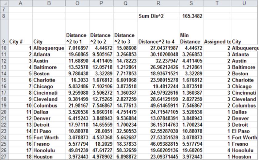
Figure 23-7: Solver window for cluster anchors

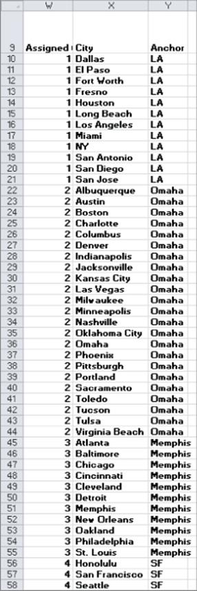
The Evolutionary Solver finds that the cluster anchors are Los Angeles, Omaha, Memphis, and San Francisco. Figure 23.8 shows the members of each cluster.

Figure 23-8: Assignment of cities to clusters

Interpretation of Clusters

The z-scores of the anchors represent a typical member of a cluster. Therefore, examining the z-scores for each anchor enables you to easily interpret your clusters.

You can find that the San Francisco cluster consists of rich, older, and highly Asian cities. The Memphis cluster consists of highly Black cities with high unemployment rates. The Omaha cluster consists of average income cities with few minorities. The Los Angeles cluster consists of highly Hispanic cities with high unemployment rates.

From your clustering of U.S. cities a company like Procter & Gamble that often engages in test marketing of a new product could now predict with confidence that if a new product were successfully marketed in the San Francisco, Memphis, Los Angeles, and Omaha areas, the product would succeed in all 49 cities. This is because the demographics of each city in the data set are fairly similar to the demographics of one of these four cities.

Determining the Correct Number of Clusters

After a while, adding clusters often yields a diminishing improvement in the target cell. To determine the “correct” number of clusters, you can add one cluster at a time and see if the additional complexity of adding a cluster yields improved insights into the demographic structure of U.S. cities. You can usually start by running three clusters (see Exercise 1) and in this case you can find a Sum of Distances Squared of 212.5 with anchors of Philadelphia (corresponding to the Memphis cluster), Omaha, and San Diego (corresponding to the Los Angeles cluster). When you use four clusters, the San Francisco cluster is added, thereby reducing the Sum of Distances Squared to 165.35. This large improvement justifies the use of four clusters. If you increase to five clusters (see Exercise 2) all that happens is that Honolulu receives its own cluster and the Sum of Distances Squared decreases to 145.47. With deference to Honolulu, this doesn't justify an extra cluster, so you can stop at four clusters.

The problem of determining the correct number of clusters involves trading off parsimony against specificity. After all, you could simply choose each city as a cluster. In this case you have high specificity but no parsimony. The importance of cluster analysis is that the clusters often yield a parsimonious representation of large data sets that leads to an understanding of market segments. In your study of principal components in Chapter 37, “Principal Components Analysis (PCA),” you will again encounter the parsimony vs. specificity tradeoff.

Using Conjoint Analysis to Segment a Market

As explained in Chapter 16, “Conjoint Analysis,” you can use conjoint analysis to segment the customers in a given market. Recall from Chapter 16 that for each customer you run a regression to predict the customer's ranking of a product from the levels of each product attribute. In this section you learn how the coefficients of these regressions can be used to identify market segments.

To illustrate how cluster analysis can be used to segment the market, suppose you are a market analyst for Coca-Cola and you ask 132 soda drinkers (see the worksheet Conjoint Data in the CokePepsi.xlsx file) to rank the 20 product profiles (shown in Figure 23.9) describing a six-pack of soda.

Figure 23-9: Product profiles for Coke and Pepsi

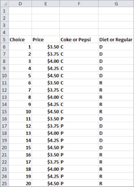
Each customer's ranking (with rank of 20 indicating the highest rated product and a rank of 1 the lowest rated product) of the 20 product profiles are in the range AC29:AW160. For example, customer 1 ranked profile 6 ($3.50 Regular Coke) highest and profile 15 ($4.50 Diet Pepsi) lowest. You can use this data and cluster analysis to segment the market.

1. Determine the regression equation for each customer. Let each row of your spreadsheet be the regression coefficients the customer gives to each attribute in the regression. Then do a cluster analysis on these regression coefficients.

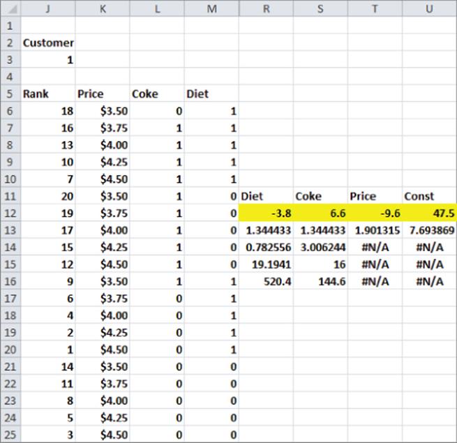
2. Next, determine the regression coefficients for each customer where the dependent variable is the customer's rank and the independent variables describe the product profile. Figure 23.10 shows the data needed to run the regression for customer 1. Coke = 1 indicates a product profile was Coca-Cola (so Coke = 0 indicates Pepsi) and Diet = 1 to indicate that a product profile was diet (so Diet = 0 indicates the product profile was regular soda).

3. Enter the customer number in cell J3. Then copy the formula =INDEX(ranks,$J$3,D6) from cell J6 to J7:J25 to pick off the customer's ranking of the product profiles. (The range ranks refers to the range AD29:AW160.)

Figure 23-10: Setting up regression for Coke-Pepsi cluster analysis

To get the regression coefficients, you need to run a regression based on each customer's rankings. Therefore you need to run 132 regressions. Combining Excel's array LINEST function with the Data Table feature makes this easy. In Chapter 10, “Using Multiple Regression to Forecast Sales,” you learned how to run a regression with the Data Analysis tool. Unfortunately, if the underlying data changes, this method does not update the regression results. If you run a regression with LINEST, the regression coefficients update if you change the underlying data.

1. To run a regression with LINEST when there are m independent variables, select a blank range with five rows and m + 1 columns. The syntax of LINEST is LINEST(knowny's,knownx's,const,stats).

2. To make any array function work you must use the Control+Shift+Enter key sequence. After selecting the cell range R12:U16 with the cursor in R12, enter =LINEST(J6:J25,K6:M25,TRUE,TRUE) and the array enters the formula with the Control+Shift+Enter key sequence.

3. Now in R12:U12 you can find the least-squares regression equation; with the coefficients read right to left, starting with the Intercept. For example, for customer 1 the best fit to her rankings is 47.5 − 3.8 Diet + 6.6 Coke − 9.6 Price. This indicates that customer 1 prefers Regular to Diet and Coke to Pepsi. You do not need to be concerned with the remainder of the LINEST output.

You can now use a one-way data table to loop LINEST through each customer and track each customer's regression equation. You can do so by completing the following steps. The results are shown in Figure 23.11.

1. Enter the customer numbers in AY11:AY130. The customer numbers are the input into a one-way data table (so called because the table has only one input cell: customer number.) As you vary the customer number, the one-way data table uses the LINEST function to compute the coefficients of each customer's regression equation.

2. Copy the formula =R12 from AZ10 to BA10:BB10 to create output cells, which pick up each regression coefficient.

3. Select the Table range AY10:BB130, and select What-If Analysis from the Data Tools Group on the Data tab.

4. Next select Data Table… and as shown in Figure 23.12, choose J3 as the column input cell. This causes Excel to loop through each customer and use LINEST to run a regression based on each customer's rank.

5. Copy the regression results from your data table to the worksheet cluster, and run a cluster analysis with five clusters on the regression coefficients. Use customers 1–5 as the initial set of anchors. The results are shown in Figure 23.13.

Figure 23-11: Regression coefficients for Coke-Pepsi cluster analysis

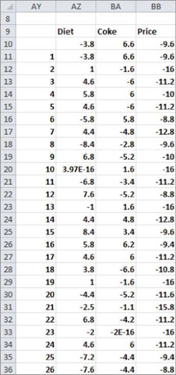
Figure 23-12: $J$3 is the column input cell for a one-way data table.

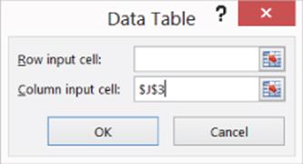
Figure 23-13: Cluster results for Coke-Pepsi cluster analysis

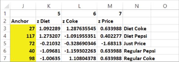
You can find the following clusters:

· The first cluster represents people with a strong preference for Diet Coke.

· The second cluster represents people with a strong preference for Diet Pepsi.

· The third cluster represents people who make their soda choice based primarily on price.

· The fourth cluster represents people who prefer Regular Pepsi.

· The fifth cluster represents people who prefer Regular Coke.

NOTE

The final target cell value for the cluster analysis was 37.92. When you run an Evolutionary Solver model multiple times, the Solver may find a slightly different target cell value. Thus in the current situation Solver might find a target cell value of, say, 38. The changing cells might also be different, but the interpretation of the cluster anchors would surely remain the same.

Summary

To construct a cluster analysis with n clusters, do the following:

· Choose n trial anchors.

· For each data point standardize each attribute.

· Find the squared distance from each anchor to each data point.

· Assign each data point the squared distance to the closest anchor.

· Increase the Mutation rate to 0.5 and use the Evolutionary Solver to minimize the Sum of the Squared Distances.

· Interpret each cluster based on the attribute z-scores for the cluster anchor.

Exercises

1. Run a three-cluster analysis on your U.S. City data.

2. Run a five-cluster analysis on your U.S City data.

3. When you ran your four-cluster U.S. City analysis, you did not put in a constraint to ensure that Solver would not pick the same city twice. Why was it not necessary to include such a constraint?

4. The file cereal.xls contains calories, protein, fat, sugar, sodium, fiber, carbs, sugar, and potassium content per ounce for 43 breakfast cereals. Use this data to perform a cluster analysis with five anchors.

5. The file NewMBAdata.xlsx contains average undergrad GPA, average GMAT score, percentage acceptance rate, average starting salary, and out of state tuition and fees for 54 top MBA programs. Use this data to perform a cluster analysis with five anchors.

6. Verify that the z-scores for each attribute in the file cluster.xlsx have a mean of 0 and a standard deviation of 1.

7. Do an Internet search for Claritas. How are Claritas's services based on cluster analysis?