Marketing Analytics: Data-Driven Techniques with Microsoft Excel (2014)
Part VI. Market Segmentation
Chapter 24. Collaborative Filtering
In today's world you have so many choices. What book should you read next? What movie should you rent? What hot, new song should you download to your iPod or iPhone? Collaborative filtering is the buzzword for methods used to “filter” choices using the collective intelligence of other people's product choices. The web has made it easy to store the purchasing history and preferences of thousands, and in some cases, millions of consumers. The question is how to use this data to recommend products to you that you will like but didn't know you wanted. If you ever rented a movie from a Netflix recommendation, bought a book from an Amazon.com recommendation, or downloaded an iTunes song from a Genius recommendation, you have used a result generated by a collaborative filtering algorithm.
In this chapter you'll see simple examples to illustrate the key concepts used in two types of collaborative filtering: user-based and item-based collaborative filtering algorithms.
User-Based Collaborative Filtering
Suppose you have not seen the movie Lincoln and you want to know if you would like it. In user-based collaborative filtering, you look for moviegoers whose rating of movies you have seen is most similar to yours. After giving a heavier weighting to the most similar moviegoers, you can use their ratings to generate an estimate of how well you would like Lincoln.
NOTE
Despite the title, Badrul Sarwar et al.'s article “Item-Based Collaborative Filtering Recommendation Algorithms” (Transactions of the Hong Kong ACM, 2001, pp. 1–11) contains a detailed discussion of user-based collaborative filtering.
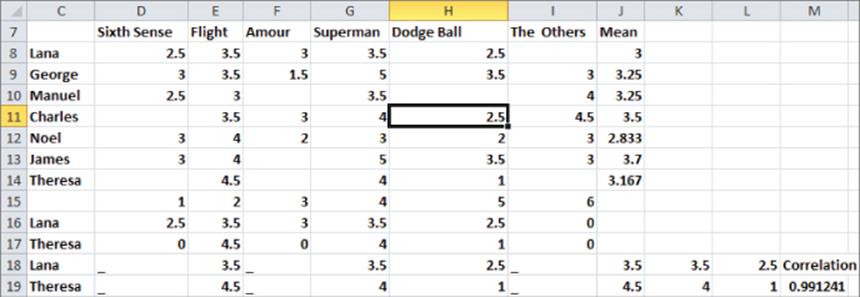
You can use the following simple example to further illustrate how user-based collaborative filtering works. Suppose seven people (Lana, George, Manuel, Charles, Noel, James, and Theresa) have each rated on a 1–5 scale a subset of six movies (Sixth Sense, Flight, Amour, Superman, Dodge Ball, and The Others). Figure 24.1 (see file finaluserbased.xlsx) shows the ratings.
Figure 24-1: Movie ratings
Now suppose you want to predict Theresa's rating for the tearjerker Amour, which she has not seen. To generate a reasonable member-based forecast for Theresa's rating for Amour, proceed as follows:
1. Begin with Theresa's average rating of all movies she has seen.
2. Identify the people whose ratings on movies seen by Theresa are most similar to Theresa's ratings.
3. Use the ratings of each person who has seen Amour to adjust Theresa's average rating. The more similar the person's other ratings are to Theresa's, the more weight you give their ratings.
Evaluating User Similarity
There are many measures used to evaluate the similarity of user ratings. You can define the similarity between two users to equal the correlation between their ratings on all movies seen by both people. Recall that if two people's ratings have a correlation near +1, then if one person rates a movie higher than average, it is more likely that the other person will rate the movie higher than average, and if one person rates a movie lower than average, then it is more likely that the other person rates the movie lower than average.
NOTE
See pp. 356–58 of Blattberg's Database Marketing, Springer, 2008 for an excellent discussion of similarity measures.
On the other hand, if two people's ratings have a correlation near −1, then if one person rates a movie higher than average, it is more likely that the other person will rate the movie lower than average, and if one person rates a movie lower than average, then it is more likely that the other person rates the movie higher than average. The Excel CORREL function can determine the correlation between two data sets. To find the correlation between each pair of moviegoers, proceed as follows:
1. In cells C16 and C17, type in the cells the names of any two moviegoers. (The worksheet Correlation sim uses Lana and Theresa.)
2. Copy the formula =INDEX($D$8:$I$14,MATCH($C16,$C$8:$C$14,0),D$15) from D16 to D16:I17 to place Lana's and Theresa's ratings in rows 16 and 17.
3. You cannot use the CORREL function on the data in rows 16 and 17 because Excel will use the 0s (corresponding to unseen movies) in its calculations. Therefore, copy the formula =IF(COUNTIF(D$16:D$17,">0") = 2,D16,"_") from D18 to D18:I19 to replace all 0s in rows 16 and 17 with a _. This ensures that when you measure similarity between two people's movie ratings via correlation you use only movies that were rated by both people.
4. Enter the formula =CORREL(D18:I18,D19:I19) in cell M19 to compute the correlation, or similarity between Lana's and Theresa's ratings. The correlation of 0.991241 indicates that Lana and Theresa have similar tastes in movies.
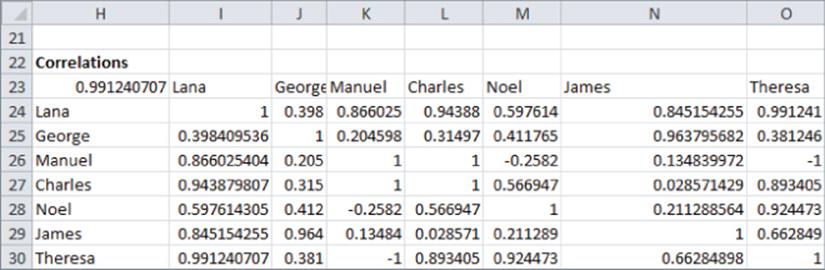
5. Now use a two-way data table to compute for each pair of people the correlations between their movie ratings. List all people's names in the ranges H24:H30 and I23:O23.
6. In H23 reenter the correlation formula =CORREL(D18:I18,D19:I19).
7. Select the table range of H23:O30, select Data Table… from the What-If portion of the Data Tools Group on the Data tab, and select C16 as the row input cell and C17 as the column input cell. This enables Excel to loop through all pairs of movie viewers and yields the correlations shown in Figure 24.2.
Figure 24-2: User similarities
Estimating Theresa's Rating for Amour
You can use the following formula to estimate Theresa's rating for Amour. All summations are for moviegoers who have seen Amour.
1 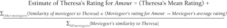
To generate your estimate of Theresa's rating for Amour, start with Theresa's average rating of all movies and use the following types of moviegoers to increase your estimate of Theresa's rating for Amour:
· People who have a positive similarity to Theresa and like Amour more than their average movie.
· People who have a negative similarity to Theresa and like Amour less than their average movie.
Use the following types of moviegoers to decrease your estimate of Theresa's rating for Amour:
· People who have a positive similarity to Theresa and like Amour less than their average movie.
· People who have a negative similarity to Theresa and like Amour more than their average movie.
The denominator of Equation 1 ensures that the sum of the absolute value of the weights given to each moviegoer adds up to 1. The calculations used to determine your estimate of Theresa's rating for Amour are as follows:
1. Copy the formula =AVERAGE(D8:I8) from J8 to J9:J14 to compute the average rating for each person. For example (refer to Figure 24.1), Theresa's average movie rating is 3.167.
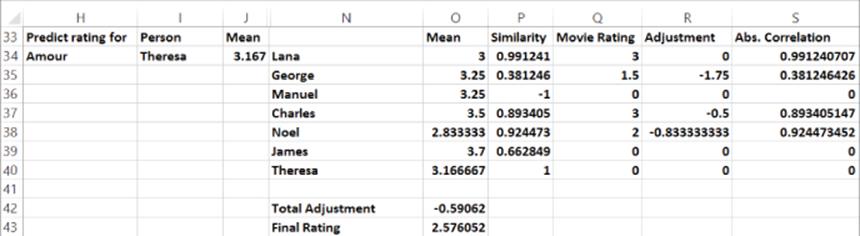
2. The remaining calculations are shown in Figure 24.3. In H34 and I34 choose (via drop-down boxes) the movie-person combination for which you want to estimate a rating.
3. Copy the formula =VLOOKUP(N34,$C$8:$J$14,8,FALSE) from O34 to O35:O40 to copy each person's average rating. For example, in cell O34 your formulas extract Lana's average rating (3).
4. Copy the formula =INDEX(correlations,MATCH($I$34,$H$24:$H$30,0),MATCH(N34,$I$23:$O$23,0)) from P34 to P35:P40 to pull the similarity of each person to the selected person. The first MATCH function ensures you pull the correlations for Theresa, whereas the second MATCH function ensures that you pull the similarity of Theresa to each other person. For example, the formula in cell P35 extracts the 0.38 correlation between George and Theresa.
5. The anchoring of H34 in the second MATCH function ensures that copying the formula =INDEX(ratings,MATCH(N34,$N$34:$N$40,0),MATCH($H$34,$D$7:$I$7,0))from Q34 to Q35:Q40 pulls each person's rating for Amour. If the person has not seen Amour, enter a value of 0. For example, the formula in Q35 extracts George's 1.5 rating for Amour.
6. Copy the formula =IF(AND(N34<>$I$34,Q34>0),(Q34-O34),0) from R34 to R35:R40 to compute for each person who has seen Amour an adjustment equal to the amount by which the person's rating for Amour exceeds their average movie rating. For example, George gave movies an average rating of 3.25 and rated Amour only a 1.5, so George's adjustment factor is 1.5 – 3.25 = −1.75. Anyone who has not seen Amour has an adjustment factor of 0.
7. Copy the formula =IF(AND(N34<>$I$34,Q34>0),ABS(P34),0) from S35:S40 to enter the absolute value of the correlation between Theresa and each person who has seen Amour.
8. In O42 the formula =SUMPRODUCT(R34:R40,P34:P40)/SUM(S34:S40) computes (−0.591) the second term in Equation 1, which is used to compute the total amount by which you can adjust Theresa's average rating to obtain an estimate of Theresa's rating for Amour.
9. Finally, enter the formula =J34+O42 in cell Q43 to compute your estimate (2.58) for Theresa's rating.
NOTE
You adjusted Theresa's average rating downward because George's, Charles's, and Noel's tastes were similar to Theresa's tastes, and all of them rated Amour below their average movie rating.
Figure 24-3: Estimating Theresa's rating for Amour
Item-Based Filtering
An alternative method to user-based collaborative filtering is item-based collaborative filtering. Think back to the Lincoln movie example. In item-based collaborative filtering (first used by Amazon.com) you first determine how similar all the movies you have seen are to Lincoln. Then you can create an estimated rating for Lincoln by giving more weight to your ratings for the movies most similar to Lincoln.
Now return to the Amour example, and again assume that you want to estimate Theresa's rating for Amour. To apply item-based filtering in this situation, look at each movie Theresa has seen and proceed as follows:
1. For each movie that Theresa has seen, use the correlation of the user ratings to determine the similarity of these movies to the unseen movie (Amour).
2. Use the following Equation 2 to estimate Theresa's rating for Amour.
2 
Analogously to Equation 1, Equation 2 gives more weight to the ratings on movies Theresa has seen that are more similar (in the sense of absolute correlation) to Amour. For movies whose ratings are positively correlated to Amour's rating, increase your estimate if Theresa rated the movie above her average. For movies whose ratings are negatively correlated to Amour's rating, decrease your estimate if Theresa rated the movie above her average. The worksheet Correlation sim in the file finalitembasednew.xlsx contains calculations of an estimate of Theresa's rating for Amour. The calculations proceed as follows:
1. In C16 and C17 use the drop down box to enter any two movies.
2. Copy the following formula from D16 to D16:I17 to extract each person's rating for the two selected movies Note that if a person did not rate a movie a - is entered.
=IF(INDEX($D$8:$I$14,D$15,MATCH($C16,$D$7:$I$7,0))=0,"-",INDEX($D$8:$I$14,D$15,MATCH($C16,$D$7:$I$7,0)))
3. Copy the formula =IF(OR(D$16="-",D$17="-"),"-",D16) from D18 to D18:I19 to extract only the ratings from users who rated both movies.
4. In D22 use the formula =CORREL(D18:J18,D19:J19) to compute the correlation between the selected movies. In this case Amour and my all-time favorite comedy, Dodge Ball (by the way if you like Dodge Ball you will love We're the Millers), have a −0.49 correlation.
5. As shown in Figure 24.4, use a two-way data table (row input cell of C16 and column input cell of C17) to compute in the cell range N22:T27 the correlation between each pair of movies.
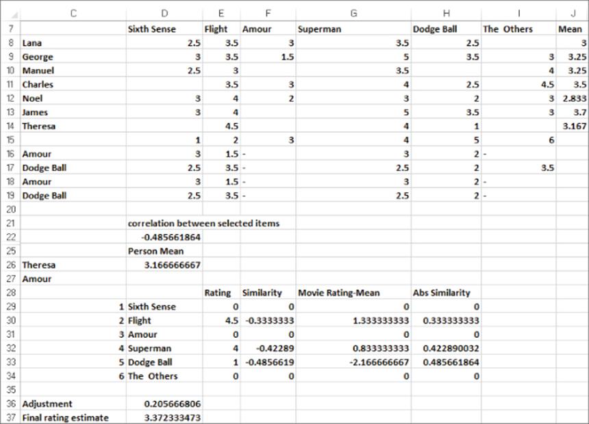
6. In C26 and C27 use the drop down boxes to select the person (Theresa) and the movie (Amour) for which you want to predict an estimated rating. The range C28:H37 shown in Figure 24.5 contains the final calculations used to generate your item-based prediction for Theresa's rating ofAmour.
7. Copy the formula =INDEX($D$8:$I$14,MATCH($C$26,$C$8:$C$14,0),MATCH($D29,$D$7:$I$7,0)) from E29 to E30:E34 to extract Theresa's rating for each movie. (A 0 indicates an unrated movie.) For example, the formula in cell E30 extracts Theresa's rating of 4.5 for Flight while E29 contains a 0 because Theresa did not see Sixth Sense.
8. Copy the formula =IF(E29=0,0,INDEX($O$22:$T$27,MATCH($C$27,$O$21:$T$21,0),MATCH(D29,$O$21:$T$21,0))) from F29 to F30:F34 to extract for each movie Theresa has seen the correlation of the movie's ratings with Amour's ratings. For example, cell F30 contains the correlation between Flight and Amour (−0.33) while F29 contains a 0 because Theresa did not see Sixth Sense.
9. Copy the formula =IF(E29=0,0,E29-$D$26) from G29 to G30:G34 to compute for each movie Theresa has seen the amount by which Theresa's rating for a movie exceeds her average rating. For example, Theresa's rating of 4.5 for Flight exceeded her average rating of 3.17 by 1.33, which is the result shown in G30.
10. Copy the formula =ABS(F29) from H29 to H30:H34 to compute the absolute value of the correlation of each movie's rating with Amour's ratings.
11. In cell D36 use the formula =SUMPRODUCT(G29:G34,F29:F34)/SUM(H29:H34) to compute the second term “adjustment” from Equation 2 to generate Theresa's estimated rating for Amour. You should increase Theresa's average rating of 3.167 by 0.21.
12. In cell D37 use Equation 2 to compute the final estimate (3.37) of Theresa's rating (3.37) for Amour with the formula =D26+D36. If you select a different movie and a different person in C26 and C27, then cell D37 will contain your estimate of that person's rating for the movie.
Figure 24-4: Item correlations
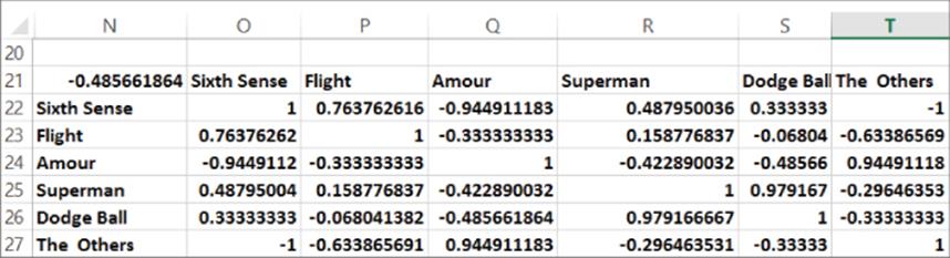
Figure 24-5: Using item-based filtering to estimate Theresa's rating for Amour
Comparing Item- and User-Based Collaborative Filtering
In the past, user-based collaborative filtering was often used because it was easy to program (Sarwar et al., 2001). User-based collaborative filtering also tends to be more attractive in situations where users are personally familiar with each other. A good example would be if Facebook was trying to provide you with music recommendations based on the preferences of your Facebook friends. With user-based filtering Facebook could provide you with a list of your friends whose musical preferences were most similar to yours.
Companies with many customers who aren't necessarily familiar with one another, such as Amazon.com, prefer the item-based approach to the user-based approach because the item-based matrix of correlations is more stable over time than the user-based matrix of correlations and therefore needs to be updated less frequently. Also, when user-based collaborative filtering is applied to a situation in which there are many customers and products, the calculations do become increasingly more burdensome than the calculations associated with the item-based approach.
The Netflix Competition
Perhaps the best-known example of collaborative filtering was the Netflix Prize Competition, which began in October 2006. Netflix made public more than 100 million movie ratings (the training set) and withheld 1.4 million ratings (the test set) from the competitors. Accuracy of a forecasting algorithm was measured by Root Mean Squared Error (RMSE). Letting N = Number of ratings in the test set, RMSE is defined as the following:
![]()
Netflix's algorithm had an RMSE of 0.9514. Netflix offered a $1 million prize to the first entry that beat this RMSE by at least 10 percent. In June 2009 the BellKor Pragmatic Chaos team became the first team to improve RMSE by 10 percent. BellKor won by submitting its entry only 20 minutes before the second place team! The prize-winning recommendation system was actually a combination of more than 100 algorithms. You might enjoy the excellent discussion of the Netflix prize in Chapter 4 of Mung Chiang's book, A Networked Life (Cambridge University Press, 2012).
Summary
In this chapter you learned the following:
· User-based collaborative filtering estimates a person's rating for a product by weighting most heavily the opinions of similar users.
· Item-based collaborative filtering estimates a person's rating for a product by weighting most heavily a person's ratings for products most similar to the product in question.
Exercises
The following table shows ratings for six people and six movies.
|
Movie 1 |
Movie 2 |
Movie 3 |
Movie 4 |
Movie 5 |
Movie 6 |
|
|
Jane |
5 |
4 |
||||
|
Jill |
4 |
3 |
3 |
|||
|
Britney |
5 |
5 |
4 |
5 |
4 |
4 |
|
Phil |
1 |
2 |
||||
|
Gloria |
3 |
7 |
5 |
|||
|
Mitchell |
2 |
4 |
4 |
3 |
1. Use user-based filtering to predict each missing rating in the table.
2. Use item-based filtering to predict each missing rating in the table.
3. How could the concept of a Training set be used to improve the quality of the estimated ratings defined by Equations 1 and 2?
All materials on the site are licensed Creative Commons Attribution-Sharealike 3.0 Unported CC BY-SA 3.0 & GNU Free Documentation License (GFDL)
If you are the copyright holder of any material contained on our site and intend to remove it, please contact our site administrator for approval.
© 2016-2026 All site design rights belong to S.Y.A.