Marketing Analytics: Data-Driven Techniques with Microsoft Excel (2014)
Part VI. Market Segmentation
Chapter 25. Using Classification Trees for Segmentation
In Chapter 23, “Cluster Analysis,” you learned how cluster analysis can be used to determine market segments. Often the marketing analyst wants to develop a simple rule for predicting whether a consumer will buy a product. You can use decision trees to determine simple classification rules that can be understood by people with little statistical training. For example, Market Facts of Canada Limited (see http://www.quirks.com/articles/a1993/19930206.aspx?searchID=30466011) wanted to determine a simple rule that could be used to predict whether a family was likely to purchase a Canadian savings bond. It used a decision tree to show that the best predictor of bond ownership was annual household income in excess of $50,000, with the second best predictor being the region in which the family resided.
This chapter discusses decision trees and how you can use them to develop simple rules that can be used to predict the value of a binary dependent variable from several independent variables.
Introducing Decision Trees
Decision trees are used to predict a categorical (usually binary) dependent variable such as:
· Will a family purchase a riding mower during the next year?
· Will a person suffer a heart attack in the next year?
· Will a voter vote Republican or Democratic in the next presidential election?
NOTE
See Victory Lab (by Sasha Issenberg, Random House, 2012) for a discussion of how decision trees were used in Obama's successful 2012 reelection campaign.
Similar to logistic regression (see Chapter 17, “Logistic Regression”), you can try and determine the independent variables or attributes that are most effective in predicting the binary dependent variable. You begin the tree with a root node that includes all combinations of attribute values, and then use an independent variable to “split” the root node to create the most improvement in class separation.
To understand the basic idea of class separation, suppose you want to predict whether a family will buy a riding mower. If every family owning a lot of at least 2 acres in size bought a riding mower and no family owning a lot less than 2 acres in size bought a riding mower, then you could split the root node into two child nodes: one with Lot Size <2 acres and another with Lot Size ≥2 acres, and you would have a simple, perfectly performing classification rule: if Lot Size ≥2 acres, predict a family will buy a riding mower, and if Lot Size <2 acres, predict a family will not buy a riding mower. If the first split does not result in a satisfactory classification performance, then you split the two child nodes, possibly on another independent variable. Eventually a satisfactory but simple to understand classification rule is obtained.
You can see this concept more clearly using a simple example to illustrate the construction of a decision tree.
Constructing a Decision Tree
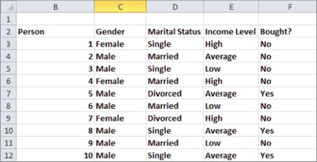
Suppose that you want to come up with a simple rule to determine whether a person will buy Greek yogurt. Figure 25.1 contains data on a sample of 10 adults (see the Greekyogurt.xlsx file). For example, Person 1 is a single, high-income woman who did not buy Greek yogurt. In this example the dependent variable for each person is whether or not the person purchased Greek yogurt.
Figure 25-1: Data on Greek yogurt purchasers
A node of a decision tree is considered pure if all data points associated with the node have the same value of the dependent variable. You should branch only on impure nodes. In this example, because the root node contains three purchasers of yogurt and seven nonpurchasers, branch on the root node. The goal in branching is to create a pair of child nodes with the least impurity.
There are several metrics used to measure the impurity of a node. Then the impurity of a split is computed as a weighted average of the impurities for the nodes involved in the split, with the weight for a child node being proportional to the number of observations in the child node. In this section you use the concept of entropy to measure the impurity of a node. In Exercises 1 and 2 you explore two additional measures of node impurity: the Gini Index and classification error.
To define the entropy of a node, suppose there are c possible values (0, 1, 2, c-1) for the dependent variable. Assume the child node is defined by independent variable X being equal to a. Then the entropy of the child node is computed as the following equation:
1 ![]()
In Equation 1 the following is true:
· P(i|X = a) is the fraction of observations in class i given that X = a.
· Log2 (0) is defined to equal 0.
Entropy always yields a number between 0 and 1 and is a concept that has its roots in Information Theory. (See David Luenberger's Information Science, Oxford University Press, 2006 for an excellent introduction to Information Theory.) With two classes, a pure node has an entropy of 0 (−0*Log2 0 + 1*Log2 1) = 0). A split of a node can yield a maximum entropy value of 1 when one-half the observations associated with a node have c = 0 and c = 1 (see Exercise 5). This shows that intuitively picking a split based on entropy can yield pure nodes. It can also be shown that with two nodes the entropy decreases as the fraction of nodes having c = 1 or c = 0 moves away from 0.5. This means that choosing splits with lower entropy will have the desired effect of decreasing impurity.
Suppose there are S possible values (s = 1, 2, …, S) for the attribute generating the split and there are ni observations having the independent variable = i. Also assume the parent node has N total observations. Then the impurity associated with the split is defined by the following equation:
2 ![]()
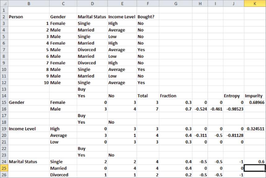
For this example suppose that you split the root node based on gender. From Equation 1 you can find that:

Because the data set contains three women and seven men Equation 2 shows you that the impurity of the split is (3 / 10) * 0 + (7 / 10) * (0.985) = 0.69.
You should split on the independent variable whose child nodes yield the lowest level of impurity. Using the Excel COUNTIFS function, it is easy to compute the level of impurity resulting from a split on each independent variable (see Figure 25.2 and the file Greekyogurt.xlsx). Then you split the root node using the independent variable that results in the lowest impurity level.
Figure 25-2: Impurity calculations from each split
Proceed as follows:
1. Copy the formula =COUNTIFS($C$3:$C$12,$C15,$F$3:$F$12,D$14) from D15 to D15:E16 to compute the number of females and males who buy and do not buy Greek yogurt. For example, you find four males do not buy Greek yogurt.
2. Copy the formula =COUNTIFS($E$3:$E$12,$C19,$F$3:$F$12,D$14) from D19 to D19:E21 to count the number of people for each income level that buy and do not buy Greek yogurt. For example, three average income people bought Greek yogurt.
3. Copy the formula =COUNTIFS($D$3:$D$12,$C24,$F$3:$F$12,D$14) from D24 to the range D24:E26 to count how many people for each marital status buy or do not buy Greek yogurt. For example, two single people buy Greek yogurt.
4. Copy the formula =SUM(D15:E15) from F15 to the range F15:F26 to compute the number of people for the given attribute value. For example, cell F25 tells you there are four married people in the population.
5. Copy the formula =F15/SUM($F$15:$F$16) from G15 to G15:G26, to compute the fraction of observations having each possible attribute value. For example, from G16 you can find that 70 percent of the observations involve males.
6. Copy the formula =IFERROR((D15/$F15)*LOG(D15/$F15,2),0) from H15 to H15:I26 to compute for each attribute value category level combination the term P(i|X=a)*Log2(P(i|X=a). You need IFERROR to ensure that when P(i|X=a)=0 Log2(0) the undefined value is replaced by 0. In general entering IFERROR(formula, anything) will enter the value computed by the formula as long as the formula does not return an error. If the formula does return an error, IFERROR returns whatever is entered after the comma (in this case 0.)
7. Copy the formula =SUM(H15:I15) from J15 to J15:J26 to compute via Equation 1 the entropy for each possible node split.
8. Copy the formula =−SUMPRODUCT(G15:G16,J15:J16) from K15 to K16:K24 to compute via Equation 2 the impurity for each split.
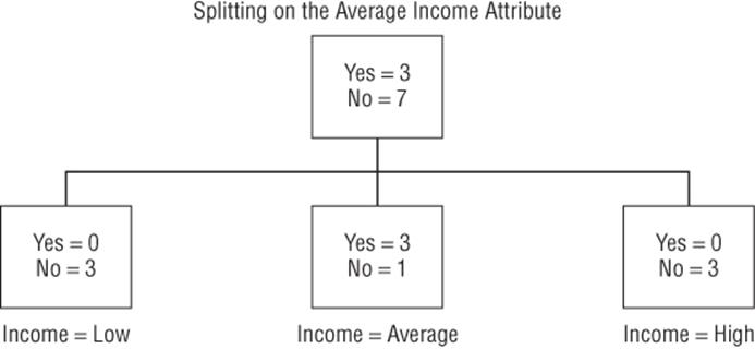
9. The impurity for income of 0.325 is smaller than the impurities for gender (0.69) and marital status (0.60), so begin the tree by splitting the parent node on income. This yields the three nodes shown in Figure 25.3. Note that this figure was drawn and was not created by Excel.
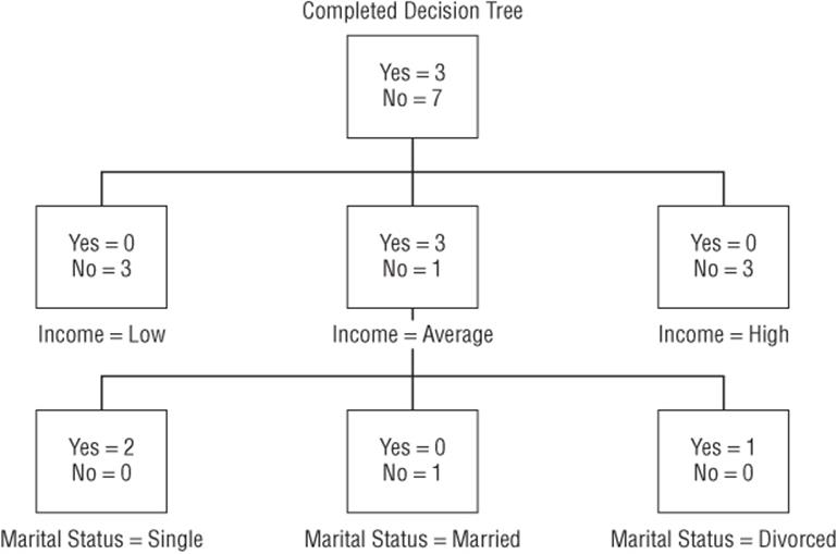
10. The Income = Low and Income = High nodes are pure, so no further splitting is necessary. The Income = Average is not pure, so you need to consider splitting this node on either gender or marital status. Splitting on gender yields an impurity of 0.811, whereas splitting on marital status yields an impurity of 0. Therefore, split the Income = Average node on marital status. Because all terminal nodes are pure (that is, each respondent for a terminal node is in the same class), no further splitting is needed, and you obtain the decision tree, as shown in Figure 25.4.
Figure 25-3: Splitting root node with Income variable
Interpreting the Decision Tree
The decision tree, shown in Figure 25.4, yields the following classification rule: If the customer's average income is either low or high, the person will not buy Greek yogurt. If the person's income is average and the person is married, the person will not buy Greek yogurt. Otherwise, the person will buy Greek yogurt. From this decision tree the marketing analyst learns that promotional activities and advertising should be aimed at average income single or divorced customers, otherwise those investments will likely be wasted.
Figure 25-4: Tree after marital status and income splits
How Do Decision Trees and Cluster Analysis Differ?
The astute reader might ask how cluster analysis (discussed in Chapter 23) and decision trees differ. Recall in Chapter 23 you divided U.S. cities into four clusters. Suppose you want to determine the cities in which a new product is likely to sell best. The clustering in Chapter 23 does not help you make predictions about sales in each city. The decision tree approach enables you to use demographic information to determine if a person is likely to buy your product. If a decision tree analysis showed you, for example, that older, high income Asian-Americans were likely to buy the product, then your Chapter 23 cluster analysis would tell you that your product is likely to sell well in Seattle, San Francisco, and Honolulu.
Pruning Trees and CART
Extensive calculation is required to create decision trees. Fortunately, widely used statistical packages such as SAS, STATISTICA, R, SPSS, and XLMINER can quickly churn out decision trees. SPSS, for example, uses Leo Breiman's (Classification and Regression Trees, Chapman and Hall, 1984) CART algorithm to generate decision trees. A key issue in creating a decision tree is the size of the tree. By adding enough nodes you can always create a tree for which the terminal nodes are all pure. Unfortunately, this usually results in overfitting, which means the tree would do poorly in classifying out of sample observations. CART “prunes” a tree by trading off a cost for each node against the benefit generated by the tree. The benefit derived from a tree is usually measured by the misclassification rate. To compute the misclassification rate for a tree, assume at each terminal node all observations are assigned to the class that occurs most frequently. All other observations associated with a node are assumed to be misclassified. Then the misclassification rate is the fraction of all misclassified observations. To illustrate the calculation of the misclassification rate, compute the misclassification rate for the tree, as shown in Figure 25.5.
Figure 25-5: Tree for illustrating misclassification rate
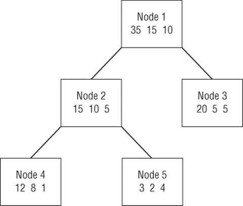
For each terminal node the number of misclassified observations is computed as follows:
· For Node 3, 20 observations are classified in Class 1, 5 in Class 2, and 5 in Class 3. For misclassification purposes you should assume that all Node 3 observations should be classified as Class 1. Therefore 10 observations (those classified as Class 2 or 3) are assumed to be misclassified.
· Node 4 observations are classified as Class 1, so the 9 observations classified as Class 2 or 3 are misclassified.
· Node 5 observations are classified as Class 3, so the 5 observations classified as Class 1 or 2 are misclassified.
· In total 24/60 = 40 percent of all observations are misclassified.
Summary
In this chapter you learned the following:
· You can use decision trees to determine simple classification rules that can be understood by people with little statistical training.
· To create a decision tree, split a parent node using a division of attribute values that creates the greatest reduction in overall impurity value.
· The widely used CART algorithm uses pruning of a decision tree to avoid overfitting and creates effective parsimonious classification rules.
Exercises
1. The Gini Index measure of impurity at a node is defined as the following:
![]()
(a) Show that when there are two classes the maximum impurity occurs when both classes have probability .5 and the minimum impurity occurs when one class has probability 1.
(b) Use the Gini Index to determine the first node split for the Greek yogurt example.
2. The classification error measure at a node is 1–maxi(P(Class=i|X=a)).
(a) Show that when there are two classes the maximum impurity occurs when both classes have equal probability and the minimum impurity occurs when one class has probability 1.
(b) Use the classification error measure to determine the first node split for the Greek yogurt example.
3. Show that when there are two classes the maximum entropy occurs when both classes have equal probability and the minimum entropy occurs when one class has probability 1.
4. How could L.L. Bean use classification trees?
5. Suppose you want to use age and tobacco use statistics to develop a decision tree to predict whether a person will have a heart attack during the next year. What problem would arise? How would you resolve this problem?
6. For the Greek yogurt example verify that if the parent node is Income = Average then splitting on gender yields an impurity of 0.811, whereas splitting on marital status yields an impurity of 0.
7. Explain how the Obama campaign could have used decision trees.
All materials on the site are licensed Creative Commons Attribution-Sharealike 3.0 Unported CC BY-SA 3.0 & GNU Free Documentation License (GFDL)
If you are the copyright holder of any material contained on our site and intend to remove it, please contact our site administrator for approval.
© 2016-2026 All site design rights belong to S.Y.A.