Marketing Analytics: Data-Driven Techniques with Microsoft Excel (2014)
Part VII. Forecasting New Product Sales
Chapter 27. The Bass Diffusion Model
Businesses regularly invest large sums of money in new product development. If the product does not sell well, these investments can reduce the company's value or share price. It is therefore of critical importance to predict future sales of a product before a product comes to market. The Bass model and its variants meet this challenge. Unlike the Pearl and Gompertz curves you learned about in Chapter 26, “Using S Curves to Forecast Sales of a New Product,” the Bass model has been successfully used to forecast product sales before the product comes to market. The Bass model also gives the analyst an explanation of how knowledge of new products spreads throughout the market place.
Introducing the Bass Model
The Bass model asserts that diffusion of a new product is driven by two types of people:
· Innovators: Innovators are people who seek new products without caring if other people have adopted the new product.
· Imitators: Imitators are people who wait to try a product until other people have successfully used the product.
The Bass model helps the marketing analysts determine the relative importance of innovators and imitators in driving the spread of the product. To understand the Bass model, you need to carefully develop some notation, defined as follows:
· n(t) = Product sales during period t.
· N(t) = Cumulative product sales through period t.
· ![]() = Total number of customers in market; assume that all of them eventually adopt the product.
= Total number of customers in market; assume that all of them eventually adopt the product.
· P = Coefficient of innovation or external influence.
· Q = Coefficient of imitation or internal influence.
The Bass Model asserts the following equation:
1 ![]()
Equation 1 decomposes the sales of a product during period t into two parts:
· A component tied to the number of people (![]() − N(t − 1)) who have not yet adopted the product. This component is independent of the number of people (N(t − 1)) who have already adopted the product. This explains why P is called the coefficient of innovation or external influence.
− N(t − 1)) who have not yet adopted the product. This component is independent of the number of people (N(t − 1)) who have already adopted the product. This explains why P is called the coefficient of innovation or external influence.
· A component tied to the number of interactions between previous adopters (N(t − 1)) and people who have yet to adopt (![]() s − N(t − 1)). This term represents the diffusion of the product through the market. This imitation or internal influence component reflects that previous adopters tell nonadopters about the product and thereby generate new adoptions. The imitation factor is often referred to as a network effect.
s − N(t − 1)). This term represents the diffusion of the product through the market. This imitation or internal influence component reflects that previous adopters tell nonadopters about the product and thereby generate new adoptions. The imitation factor is often referred to as a network effect.
NOTE
The imitation factor is 0 (because N(0) = 0) at time 0 and increases until N(t) = /2. P and Q are assumed to be between 0 and 1.
Estimating the Bass Model
To fit the Bass model, you must find values of P, Q, and ![]() , which accurately predict each period's actual sales (n(t)). To estimate P, Q, and
, which accurately predict each period's actual sales (n(t)). To estimate P, Q, and ![]() , use the Solver. To illustrate the estimation of the Bass model, use U.S. sales of color TVs; the file ColorTV.xls contains 16 years of color TV sales (1964–1979). Solver is used to determine the values of the Bass model parameters that best fit (in the sense of minimizing the Sum of Squared Errors) the 1964–1979 data. The work is shown in Figure 27.1.
, use the Solver. To illustrate the estimation of the Bass model, use U.S. sales of color TVs; the file ColorTV.xls contains 16 years of color TV sales (1964–1979). Solver is used to determine the values of the Bass model parameters that best fit (in the sense of minimizing the Sum of Squared Errors) the 1964–1979 data. The work is shown in Figure 27.1.
Figure 27-1: Fitting Bass model to color TV data
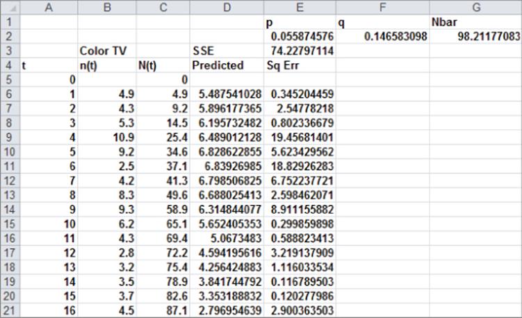
For example when t = 1 (in 1964), 4.9 million color TVs were sold. Through 1965, 9.2 million color TVs were sold. To estimate P, Q, and ![]() , proceed as follows:
, proceed as follows:
1. Put trial values of P, Q, and ![]() in E2:G2 and create range names for these cells.
in E2:G2 and create range names for these cells.
2. Using the trial values of P, Q, and ![]() , create predictions for 16 years of sales by copying the formula =p*(Nbar−C5)+(q/Nbar)*C5*(Nbar−C5) from D6 to D7:D21.
, create predictions for 16 years of sales by copying the formula =p*(Nbar−C5)+(q/Nbar)*C5*(Nbar−C5) from D6 to D7:D21.
3. In E6:E21 compute the squared error (SSE) for each year by copying the formula =(B6−D6)^2 from E6 to E7:E21.
4. Compute the Sum of Squared Errors (SSE) for your predictions in cell E3 with the formula =SUM(E6:E21).
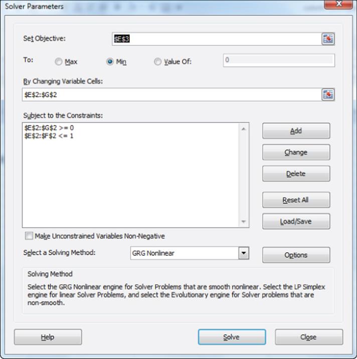
5. Use Solver's GRG Multistart Engine (see Figure 27.2) to determine values of P, Q, and ![]() that minimize SSE. P and Q are constrained to be between 0 and 1. Minimize SSE (E3) by changing P, Q, and
that minimize SSE. P and Q are constrained to be between 0 and 1. Minimize SSE (E3) by changing P, Q, and ![]() . All changing cells should be non-negative. Solver found P = .056, Q = .147, and
. All changing cells should be non-negative. Solver found P = .056, Q = .147, and ![]() = 98.21. Because Q is greater than P, this indicates that the word of mouth component was more important to the spread of color TV than the external component.
= 98.21. Because Q is greater than P, this indicates that the word of mouth component was more important to the spread of color TV than the external component.
Figure 27-2: Solver window for fitting Bass model
Fareena Sultan, John Farley, and Donald Lehmann summarized the estimated Bass model parameters for 213 products in their work “A Meta-Analysis of Applications of Diffusion Models,” (Journal of Marketing Research, 1990, pp. 70–77) and found an average value of 0.03 for P and 0.30 for Q. This indicates that imitation is much more important than innovation in facilitating product diffusion.
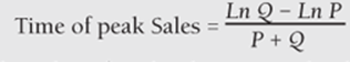
Time and Value of Peak Sales
If a product's sales are defined by Equation 1, then it follows that the time of peak sales is given by the following:
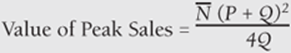
The value of peak sales is given by this equation:
Using the Bass Model to Forecast New Product Sales
It is difficult to predict the sales of a new product before it comes to market, but an approach that has proven useful in the past is to look for a similar product or industry that has already reached market maturity (for example, a color TV might be an analog for DIRECTV). Similar products or industries are often referred to as adjacent industries/categories. You can use the values of P and Q for the analogous product and an estimated value of N for the new product to forecast sales. Table 27-1 lists values of P and Q for several products.
Table 27-1: Estimates of P and Q for Bass model
|
Product |
P |
Q |
|
CD Player |
0.02836 |
0.368 |
|
Dishwasher |
0.0128 |
0.18450 |
|
Mammography |
0.00494 |
0.70393 |
|
Cell Phone |
0.00471 |
0.50600 |
|
Tractor |
0.00720 |
0.11795 |
To illustrate how you can use the Bass model to model sales of a new product, consider Frank Bass, Kent Gordon, Teresa Ferguson, and Mary Lou Githens' study “DIRECTV: Forecasting Diffusion of a New Technology Prior to a Product Launch (Interfaces, May–June 2001, pp. S82–S93), which describes how the Bass model was used to forecast the subscriber growth for DIRECTV. The discussion of this model is in file DIRECTV.xls (see Figure 27.3).
Figure 27-3: Predicting DIRECTV subscribers
Before DIRECTV was launched in 1994, the Hughes Corporation wanted to predict the sales of DIRECTV for its first four years. This estimate was needed to raise venture capital to finance the huge capital expense needed for DIRECTV to begin operations. The estimate proceeded as follows:
· Hughes surveyed a representative sample of TV households and found 32 percent intended to purchase DIRECTV.
· 13 percent of those sampled said they could afford DIRECTV.
Research has shown that intentions data greatly overstates actual purchases. A study of consumer electronics products by Linda Jamieson and Frank Bass (“Adjusting Stated Intentions Measures to Predict Trial Purchases of New Products,” Journal of Marketing Research, August 1989, pp. 336–345) showed that the best estimate of the actual proportion that will buy a product in a year is a fraction k of the fraction in the sample who say they will buy the product, where k can be estimated from the following equation:
2 ![]()
In Equation 2 Available%age is the estimated fraction of consumers who will have access to product within a year. Hughes estimated Available%age = 65%. At the time DIRECTV was introduced, there were 95 million TV households. Therefore Hughes' forecast for DIRECTV subscribers 1 year after launch is computed in cell A13 as 0.32 * 95 * (−0.899 + (1.234)(0.13) + (1.203)(0.65)) = 1.32 million.
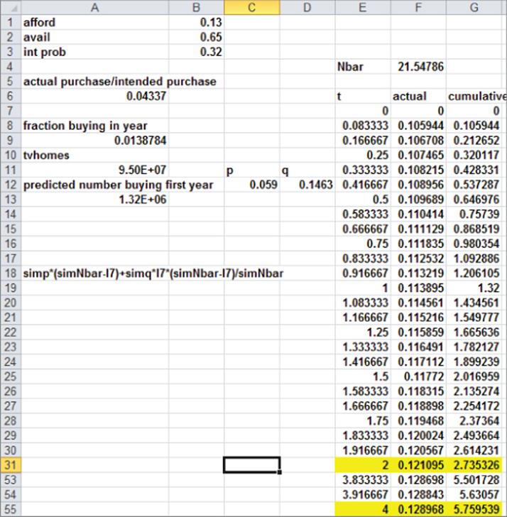
Now assume subscriptions to DIRECTV will follow the Bass model. You can generate the forecasts using color TV as the analogous product. Bass et. al. use slightly different parameters (P = .059 and Q = .1463) than the ones in the following example. You do not know Nbar, but for any given value of Nbar, you can use Equation 1 to predict cumulative monthly DIRECTV subscriptions for the next 4 years. Then using Excel's Goal Seek command, you can reverse engineer a value of Nbar, which ensures that your 1-year subscription estimate for DIRECTV is 1.32 million. Then the Bass model can give you a forecast for the number of subscribers in four years. The work proceeded as follows:
1. Because at time 0 DIRECTV has 0 subscribers, enter 0 in cells F7 and G7.
2. Copy the formula =(1/12)*(p*(Nbar-G7)+q*G7*(Nbar-G7)/Nbar) from F8 to F9:F55 and use Equation 1 to generate estimates for the number of new subscribers during each month. The (1/12) adjusts the annual P and Q values to monthly values.
3. Copy the formula =G7+F8 from G8 to G9:G55 to compute the cumulative number of subscribers as previous cumulative subscribers + new subscribers during the current month.
4. Use the Excel Goal Seek command to determine the value of Nbar that makes your 1-year estimate (in cell G19) of DIRECTV subscribers equal to 1.32 million. From the What-If portion of the Data tab, select Goal Seek . . . and fill in the dialog box, as shown in Figure 27.4.
Figure 27-4: Using Goal Seek to estimate Nbar
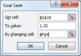
The Goal Seek window tells Excel to find the value for cell $F$4 (which is Nbar) that makes your 1-year subscriber estimate (cell $G$19) equal to 1.32 million. In the blink of an eye, Excel plugs different numbers into cell $F$4 until $G$19 equals 1.32. Nbar = 21.55 million to make your 1-year Bass forecast match your previous 1-year forecast of 1.32 million subscribers.
Cell G55 contains your 4-year forecast (5.75 million) for the number of DIRECTV subscribers. The forecast was that after four years approximately 6 percent of the 95 million homes would have DIRECTV. In reality after four years, DIRECTV ended up with 7.5 percent of the 95 million homes.
When you use the Bass model to forecast product sales based on an analogous product like this, you are applying the concept of empirical generalization. As defined by Frank Bass in “Empirical Generalizations and Marketing Science: A Personal View” (Marketing Science, 1995, pp. G6–G19.), an empirical generalization is “a pattern or regularity that repeats over different circumstances and that can be described simply by mathematical, graphical, or symbolic methods.” In this case, you have successfully forecasted DIRECTV sales before launch by assuming the pattern of new product sales, defined by the Bass model for an adjacent product (color TV), will be useful in predicting early sales for DIRECTV.
Deflating Intentions Data
The approach to estimating the rollout of DIRECTV subscribers was highly dependent on having an estimate of subscribers 1 year from now. Often such an estimate is based on intentions data derived from a survey in which consumers are asked to rank their likelihood of purchasing a product within 1 year as follows:
· Definitely buy product
· Probably buy product
· Might or might not buy product
· Probably not buy product
· Definitely not buy product
Jamieson and Bass (1989) conducted meta-analysis of intentions surveys for many products that enabled the marketing analyst to “deflate” intentions data and obtain a realistic estimate of a new product's market share after 1 year. The results are summarized in the file Marketsharedeflator.xlsx(see Figure 27.5).
Figure 27-5: Deflating intentions data
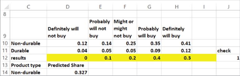
To use this market share deflator, you must first identify in cell C14 the product as a durable good (such as a car or TV) or a nondurable good (such as a frozen food dinner or new cosmetic). Note that for a durable good only 12 percent of those who say they will definitely buy actually buy, and for a nondurable good 41 percent of those who say they will definitely buy will actually buy. This is probably because durable goods are generally more expensive. Then the analyst enters the fraction of consumers who chose each option (in this case 30 percent said they will definitely buy, 40 percent said they will probably buy, 20 percent said they might or might not buy, and 10 percent said they probably will not buy). Then cell D14 tells you that your predicted market share in 1 year is 32.7 percent. Even though 70 percent of consumers gave a positive response, you can predict only a 32.7 percent share after 1 year.
Using the Bass Model to Simulate Sales of a New Product
In reality the sales of a new product are highly uncertain, but you can combine the Bass model with your knowledge of Monte Carlo simulation (see Chapter 21, “Customer Value, Monte Carlo Simulation and Marketing Decision Making”) to generate a range of outcomes for sales of a new product. Recall that Monte Carlo simulation can be used to model uncertain quantities and then generate a range of outcomes for the uncertain situation. In the Bass model the uncertain quantities are Nbar (which you model as a normal random variable) and P and Q. You will assume the values ofP and Q are equally likely to be drawn from a set of analogous products. For example, if you were a brand manager for Lean Cuisine, you could model the uncertain values of P and Q as equally likely to be drawn from the parameter values for Lean Cuisine meals that have been on the market for a number of years.
The work for the following example is in the file Basssim.xls (see Figure 27.6). In C6:D17 you are given 12 potential scenarios for Bass parameters, and you can assume potential market size is normal with mean = 100,000 and sigma = 20,000.Then proceed as follows:
1. In cell C4 simulate potential market size with the formula =ROUND(NORMINV(RAND(),C2,C3),0).
2. In cell H1 choose a scenario that chooses your Bass parameters from one of the 12 analogous products with the formula =RANDBETWEEN(1,12).
3. In cell H2 find the simulated value of P for your chosen Bass scenario with the formula =VLOOKUP(scenario,B6:D17,2).
4. Change the 2 to a 3 in cell H3 to find the simulated value of Q for your chosen Bass scenario.
5. Copy the formula =SUM($H$6:H7) from I7 to I8:I18 to compute cumulative product sales for each year. Of course, you need to enter a 0 in cell I6.
6. Copy the formula =simp*(simNbar-I6)+simq*I6*(simNbar-I6)/simNbar from H7 to H8:H18 to compute simulated sales for each year.
7. Following the technique introduced in Chapter 21, use a one-way data table to trick Excel into simulating 1,000 times your 1-year, 5-year, and 10-year cumulative sales.
8. In cells F22, G22, and H22, refer to the 1-year (I7), 5-year (I11), and 10-year (I16) sales.
9. After selecting the table range E22:H1022, choose Data Table . . . from the What-If section on the Data tab.
10. Now select any blank cell as the Column Input cell to simulate 1,000 times the 1-year, 5-year, and 10-year cumulative sales.
11. Copy the formula =AVERAGE(F23:F1022) from F20 to G20:H20 to compute an estimate of the average sales through years 1, 5, and 10.
12. Copy the formula =STDEV(F23:F1022) from F21 to G21:H21 to compute and estimate the average sales through years 1, 5, and 10.
Figure 27-6: Bass model simulation
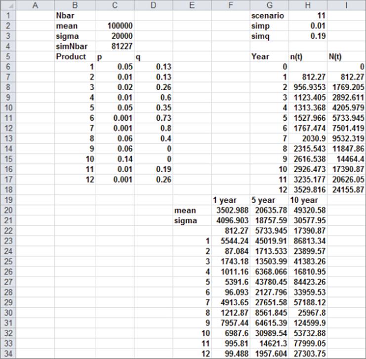
Estimates of new product sales are an important input into capital budgeting analyses, which determine if a new product should be scrapped or brought to market. You can estimate, for example, that after 5 years an average of 20,636 units will have been sold.
Modifications of the Bass Model
Since the Bass model was first introduced in 1969, the model has been modified and improved in several ways. The following list provides some important modifications of the Bass model.
· Due to population growth, the size of the market may grow over time. To account for growth in market size, you may assume that ![]() is growing over time. For example, if market size is growing 5 percent a year, you can assume that
is growing over time. For example, if market size is growing 5 percent a year, you can assume that ![]() (t) = N(0)*1.05t in Year t forecast and have Solver solve for N(0).
(t) = N(0)*1.05t in Year t forecast and have Solver solve for N(0).
· Clearly changing a product's price or level of advertising will have an impact on product sales. The Bass model has been generalized to incorporate the effects of price and advertising on sales by making P and Q dependent on the current level of price and advertising.
· For many products (such as automobiles, refrigerators, etc.), customers may return to the market and purchase a product again. To incorporate this reality, the Bass model has been modified by adjusting . ![]() For example, if people tend to buy a product every five years, you can adjust
For example, if people tend to buy a product every five years, you can adjust ![]() (t) to include people who bought a product 5 years ago.
(t) to include people who bought a product 5 years ago.
· For quarterly or monthly sales data, Equation 1 can be adjusted for seasonality. See Exercise 5.
· If a new-generation product (like an improved smartphone) is introduced, then an analog of Equation 1 is needed for both the improved and old product.
· You can make P and or Q depend on time. For example, you could allow ![]() where k and μ are parameters that can be used to allow the word of mouth factor to either increase, decrease, or remain constant over time. This model is known as the flexible logistic model.
where k and μ are parameters that can be used to allow the word of mouth factor to either increase, decrease, or remain constant over time. This model is known as the flexible logistic model.
If you want to learn more about these modifications and improvements to the Bass model, refer to New-Product Diffusion Models by Vijay Mahajan, Eitan Muller, and Yoram Wind (Springer, 2001).
Summary
In this chapter you learned the following:
· The Bass model breaks down product sales into an innovation (P) and imitation (Q) factor.
· The GRG Multistart Solver Engine can be used to estimate P, Q, and ![]() .
.
· By using an analogous product to estimate P and Q and intentions data to estimate ![]() , you can use the Bass model to estimate new product sales before the product is launched.
, you can use the Bass model to estimate new product sales before the product is launched.
· By randomly drawing values of P and Q from a set of analogous products and modeling ![]() as a normal random variable, you can simulate the range of possible product sales.
as a normal random variable, you can simulate the range of possible product sales.
Exercises
1. The file Dishwasher.xlsx contains product sales for dishwashers in the United States. Fit the Bass model to this data.
2. Fit the Bass model to the data in the file Worldcell.xslx.
Exercises 3–5 use the Chapter 26 file Internet2000_2011.xls.
3. Fit the Bass model to the Nigeria Internet data in Chapter 26.
4. Fit the Bass model to the Sweden Internet data in Chapter 26.
5. Explain the differences in the P and Q values you found in Exercises 2–4.
6. For the iPodseasonal.xls data file in Chapter 26, incorporate seasonality and fit a Bass model to the quarterly IPOD sales.
7. Suppose you work for a company that produces frozen food dinners and have found that for “traditional” dinners (mac and cheese, fried chicken, and so on) the Bass model has P near 1 and Q near 0, and for “new wave” dinners (tofu, seaweed, and such), the Bass model has P near 0 andQ near 1. How would this information affect your marketing strategy?
8. Suppose you wanted to determine whether products diffuse more quickly in developed or developing countries. Outline how you would conduct such a study.
9. Determine if the following statement is True or False: As Q/P increases, the trajectory of product diffusion becomes more S-shaped.
All materials on the site are licensed Creative Commons Attribution-Sharealike 3.0 Unported CC BY-SA 3.0 & GNU Free Documentation License (GFDL)
If you are the copyright holder of any material contained on our site and intend to remove it, please contact our site administrator for approval.
© 2016-2026 All site design rights belong to S.Y.A.