Marketing Analytics: Data-Driven Techniques with Microsoft Excel (2014)
Part VIII. Retailing
Chapter 31. Using the SCAN*PRO Model and Its Variants
Retailers have many available strategies that can be used to increase profits, including price adjustments, product placement on display, advertising, and so on. The difficulty in determining the profit-maximizing mix of marketing strategies is that factors such as seasonality and just plain random variation can make it difficult to isolate how changes in the marketing mix affect unit sales. In this chapter, you learn how to use the GRG (Generalized Reduced Gradient) multistart Solver Engine to develop forecasting models estimate variants of the SCAN*PRO model that tell the retailer how each portion of the marketing mix affects sales. Once firms understand how all these factors influence sales, they can more efficiently allocate resources to the factors that they control. Firms can also understand how external factors that they cannot control (such as competitor's price, seasonality, competitor's product on display, and so on) hinder the firm's effectiveness.
Introducing the SCAN*PRO Model
Suppose you want to predict weekly sales of Snickers (the world's best-selling candy bar) at your local supermarket. Factors that might influence sales of Snickers include:
· Price charged for Snickers bars
· Prices charged for competitors (Three Musketeers, Hershey's Chocolate, and so on)
· Was the Snickers bar on display?
· Was there a national ad campaign for Snickers?
· Was there an ad for Snickers in the local Sunday paper?
· Seasonality: Perhaps Snickers sell better in the winter than the summer.
Untangling how these factors affect unit sales of Snickers is difficult. In his paper “A Model to Improve the Baseline Estimation of Retail Sales,” (1988, see http://centrum.pucp.edu.pe/adjunto/upload/publicacion/archivo/1amodeltoimprovetheestimationofbaselineretailsales.pdf) Dirk Wittink et al. developed the widely used SCAN*PRO model to isolate the effect of these (and other factors) on sales of retail goods. The SCAN*PRO model and its variants (see Dirk Wittink et al. Building Models for Marketing Decisions, Kluwer Publishing, 2000) have been widely used by A.C. Nielsen and other organizations to analyze retail sales.
Modeling Sales of Snickers Bars
The SCAN*PRO model is often used to model the impact of various portions of the marketing mix. To predict sales you can model the effect of each part of the marketing mix as described in this section's example and create a final prediction for sales. You do this by multiplying together the terms for each part of the marketing mix and throwing in a constant to correctly scale your final prediction.
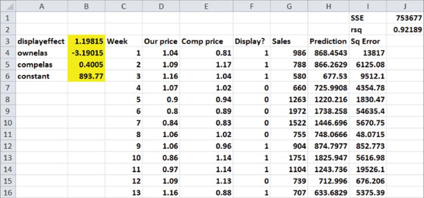
To create this model you can use the data from the Snickers.xlsx file that shows the weekly sales of Snickers bars at a local supermarket as well as the Snickers price, the price of the major competitor, and whether Snickers is on display. A subset of the data is shown in Figure 31.1. For example, in Week 1, 986 Snickers bars were sold; the price of Snickers was $1.04; the price of the main competitor was $0.81; and Snickers was on display (1 = Snickers on display, 0 = Snickers not on display). To simplify matters assume that Snickers sales do not exhibit seasonality. As you will see later in the chapter, the assumption that seasonality is not present can easily be relaxed.
Figure 31-1: Snickers sales data
To create a model to predict weekly sales, complete the following steps:
1. Raise the price to an unknown power. (Call this power OWNELAS.) This creates a term of the form (Our Price)OWNELAS. The value of OWNELAS can estimate the price elasticity. You would expect OWNELAS to be negative. For example, if OWNELAS = −3, you can estimate that for any price you charge, a 1 percent price increase reduces demand 3 percent.
2. Raise the competitor's price to an unknown power (COMPELAS). This creates a term of the form (Comp Price)COMPELAS. The value of COMPELAS estimates a cross-elasticity of demand. You would expect COMPELAS to be positive and smaller in magnitude than OWNELAS. For example, if COMPELAS = 0.4, then a 1 percent increase in the competitor's price increases demand for Snickers (for any set of prices) by 0.4 percent.
3. Model the effect of a display by a term that raises an unknown parameter (Call it DISPLAYEFFECT.) to the power DISPLAY# (which is 1 if there is a display and 0 if there is no display). This term is of the form (DISPLAYEFFECT?)DISPLAY#. When there is a display, this term equalsDISPLAYEFFECT, and when there is no display, this term equals 1. Therefore, a value of, say, DISPLAYEFFECT=1.2 indicates that after adjusting for prices, a display increases weekly sales by 20 percent.
NOTE
In Chapter 34, “Measuring the Effectiveness of Advertising,” you learn how to model the effect of advertising on sales.
Putting it all together, the final prediction for weekly sales is shown in Equation 1:
1 
You can now use the GRG multistart Solver Engine to determine values of CONSTANT, OWNELAS, COMPELAS, and DISPLAYEFFECT that minimize the sum of the squared weekly prediction errors. Proceed as follows:
1. Copy the formula =constant*(D4^ownelas)*(E4^compelas)*(displayeffect^F4) from H4 to H5:H45 to use Equation 1 to create a forecast for each week's demand.
2. Copy the formula =(G4-H4)^2 from I4 to I5:I45 to compute the squared error for each week's forecast.
3. In cell J1 compute the sum of the weekly squared errors with the formula =SUM(I4:I45).
4. In cell J2 compute the R-squared value between your predictions and actual sales with the formula =RSQ(G4:G45,H4:H45).
5. Using the Solver window shown in Figure 31.2, find the parameter estimates that minimize the sum of the squared forecast errors. Check Use Automatic Scaling from Options. This improves the performance of the Solver on sales forecasting models.
Figure 31-2: Snickers sales Solver window
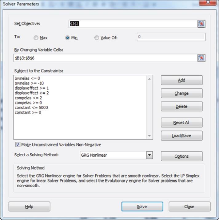
The GRG Multistart Engine requires bounds on the changing cells. Choosing “tight” bounds improves the performance of the Solver. You can assume the display effect would be between 1 and 2, the competitor's price elasticity is assumed to be between 0 and 2, the Snicker's price elasticity is assumed to be between 0 and –10, and the constant is assumed to be between 0 and 5,000. If the Solver finds a value for a changing cell near its bound, the bound should be relaxed because Solver tells you that violating the bound can probably improve your target cell.
Solver finds that the following parameters make Equation 1 a best fit for your sales data:
· The display effect = 1.198. This implied that after adjusting for prices, a Snickers display increases weekly sales by 19.8 percent.
· The price elasticity for Snickers is −3.19, so a 1 percent increase in the price of Snickers can reduce Snicker's sales by 3.19 percent.
· The cross-price elasticity for Snickers is 0.40, so a 1 percent increase in the competitor's price can raise the demand for Snickers by 0.40 percent.
Substituting your parameter values into Equation 1, you can find your prediction for weekly sales is given by:
![]()
From cell J2 you find that your model explains 92 percent of the variation in weekly sales.
Forecasting Software Sales
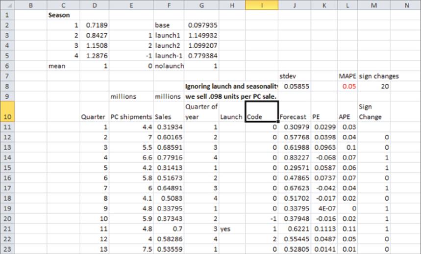
Intelligent modification of the SCAN*PRO approach can enable you to build insightful and accurate sales forecasting models that include factors other than price and product displays. To illustrate the idea, suppose you are given quarterly software sales that depend on quarterly PC shipments. Sales are seasonal and increase after a launch and drop off prior to a launch. How can you build a model to forecast sales? The work for this example is in the file softwaresales.xlsx (see Figure 31.3). Data is given for 48 quarters of software sales. For example, 700,000 units were sold in Quarter 11. During this quarter there was a software launch, the quarter was the third quarter of the year, and 4.8 million PCs were shipped.
Figure 31-3: Software sales data
The equation to forecast sales involves the following parameters:
· A seasonal index for each quarter. These seasonal indexes should average to 1. A seasonal index of, say, 1.3 for Quarter 4 means that after adjusting for other factors, sales in the fourth quarter average 30 percent more than an average quarter
· Factors (similar to the effect of the display in the Snickers example) that measure the bump up in sales the quarter of a launch (LAUNCH1) and the quarter after the launch (LAUNCH2)
· A factor (LAUNCH-1) that measures the decline in sales the quarter before a launch
· Because it seems reasonable to assume that an increase in PC shipments will increase sales of your product, you can include a term of the form BASE*PCSALES in your forecast. Here (BASE) is a changing cell that scales your forecast to minimize MAPE.
NOTE
Recall from Chapter 14, “Winter's Method,” that MAPE is the average of absolute percentage errors.
Putting it all together, your model for predicting quarterly sales (in millions) is given by Equation 2.
2 ![]()
In Equation 2, BASE is analogous to the constant term in Equation 1.
When building your sales forecasting model, you can assume that in lieu of minimizing the sum of squared errors you can minimize the average absolute percentage error (MAPE). Minimizing SSE emphasizes avoiding large outliers, and minimizing MAPE emphasizes minimizing the magnitude of the typical prediction error. Also, many practitioners prefer MAPE over SSE as a measure of forecast accuracy. This is probably because MAPE is measured as a percentage of the dependent variable, whereas it is difficult to interpret the units of SSE (in this case units2). Before using the GRG multistart Solver Engine, proceed as follows:
1. Copy the formula =base*E11*VLOOKUP(G11,lookup,2)*VLOOKUP(I11,launch,3,FALSE) from J11 to J12:J58 to compute your forecasts for all 48 quarters of data.
2. Copy the formula =(F11-J11)/F11 from K11 to K12:K58 to compute the percentage error for each quarter. For example, in Quarter 1 actual software sales were 3.0 percent higher than your prediction.
3. Copy the formula =ABS(K11) from L11 to L12:L58 to compute each week's absolute percentage error.
4. Compute the MAPE in cell L8 with the formula =AVERAGE(L11:L58).
The Solver window shown in Figure 31.4 finds the values of base, seasonal indexes, and launch effects that yield the best forecasts. The Target cell minimizes MAPE (cell L8) by changing the following parameters:
· Seasonal indices in cells D2:D5 (which must average to 1)
· A Base (in cell G2) which in effect scales PC Sales into sales of our software
· LAUNCH-1 (in cell G5) which represents the drop in sales in the quarter before a launch
· LAUNCH1 (in cell G3) which represents the increase in sales during a launch quarter
· LAUNCH2 (in cell G4) which represents the increases in sales the quarter after a launch
· The lower bound on each changing cell is 0 and the upper bound 2. The upper bound of 2 was used because it seems unlikely that sales would more than double in a quarter due to a launch and it seems unlikely that one PC sale would lead to more than two sales of the software.
Figure 31-4: Solver window for software sales

Model Interpretation
You can combine the Solver solution with Equation 2 to yield the following marketing insights:
· Quarter 4 has the highest sales with sales 29 percent better than average, and Quarter 1 has the lowest sales (28 percent below average).
· All other things being equal (ceteris paribus) the quarter of a launch, sales increase by 15 percent.
· The quarter after a launch, sales increase (ceteris paribus) by 10 percent.
· The quarter before a launch, sales decrease (ceteris paribus) by 22 percent.
· During an average quarter, an increase in PC shipments of 100 PCs leads to 9.8 more units sold.
· In cell J8 you can compute the standard deviation of percentage errors with the formula =STDEV(K11:K58). The standard deviation of 5 percent tells you that approximately 68 percent of your forecasts should be accurate within 5 percent, and approximately 95 percent of your forecasts should be accurate within 10 percent.
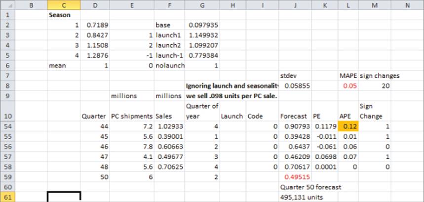
· Any quarter in which your forecast is off by 10 percent or more is an outlier. As shown in Figure 31.5, Quarter 44 is an outlier because your forecast was off by 12 percent.
Figure 31-5: Software outlier and Quarter 40 forecast
Predicting Future Sales
Assuming 6 million PC shipments in Quarter 50, suppose you are asked to forecast Quarter 50 sales and there is no launch planned in quarters 48–51. To predict Quarter 50 sales, you simply copy the forecast formula in cell J58 to J59. Your forecast for Quarter 50 sales is .495153 million or 495,153 units.
Checking for Autocorrelation
Recall from Chapter 10, “Using Multiple Regression to Forecast Sales,” that a good forecasting method should see the sign of forecast change approximately one half the time. Copying the formula =IF(K12*K11<0,1,0) from M12 to M13:M58 yields a 1 each time there is a sign change in the errors. There were 20 sign changes in the errors. The cutoff for “too few” sign changes in errors is given by ![]() = 16.6. Because 20>16.6 the forecasts exhibit random changes in sign, and no correction for autocorrelation is needed.
= 16.6. Because 20>16.6 the forecasts exhibit random changes in sign, and no correction for autocorrelation is needed.
Modeling a Trend in Sales
If you felt there was a possible trend in software sales, you could generalize Equation 2 to account for that trend. To model a trend change, change the forecast equation in J11 to Equation 3:
3 
In Equation 3, TREND is added as a changing cell. A value of TREND = 1.07 means that sales were increasing 7 percent per quarter (after adjusting for all other variables), while if TREND = 0.91 this would indicate sales were decreasing 9 percent per quarter.
Summary
In this chapter you learned the following:
· You can use the GRG multistart Solver Engine to determine how aspects of the marketing mix impact retail sales.
· The effect of your product's price can be modeled by a term of the form (Your Price)OWNELAS. The value of OWNELAS can estimate your price elasticity.
· The effect of a competitor's price can be modeled by a term of the form (Comp Price)COMPELAS. The value of COMPELAS estimates a cross-elasticity of a demand set of prices by 0.4 percent.
· The effect of a display can be modeled by a term of the form (DISPLAYEFFECT?)DISPLAY#.
· Seasonality can be incorporated into forecasts by multiplying the seasonal index by the terms involving the marketing mix.
· Other factors such as a trend and the effect of a product launch can also be incorporated in forecast models.
Exercises
1. The file Cranberries.xlsx includes quarterly sales in pounds of cranberries at a supermarket, price per pound charge, and the average price charged by competition.
(a) Use this data to determine how seasonality, trend, and price affect quarterly sales.
(b) Use a Multiplicative Model for seasonality. (The average of seasonal indexes should equal 1.)
(c) Introduce a trend and set up the model so that you can estimate price elasticity.
(d) If you charge $5 a pound in Q1 2012 and the competitor charges $5 per pound, predict the Q1 2012 sales.
(e) Fill in the blank: You are 95 percent sure the Q1 2012 sales are between _____ and ___.
Problems 2–4 use the workbook Snickers.xlsx.
2. If Snickers had more than one major competitor, how would you modify the forecast model?
3. If Snickers knew whether the competitor's product was on display, how could the model be modified?
4. Suppose you believe that if Snickers had cut its price at any time in the last four weeks, the consumer would become more price-sensitive. How would you incorporate this idea into your forecast?
5. The file POSTITDATA.xlsx contains daily information on sales of Post-it Notes. A sample of this data is shown in Figure 31.6.
Figure 31-6: Post-it sales data forecast

The following factors influence daily sales:
· Month of the year
· Trend
· Price (Seven different prices were charged.)
· Whether product is on display (1 = display, 0 = no display)
(a) Build a model to forecast daily sales. Hint: Look at the values of price that are charged. Why is a model including terms of the form (Price)elasticity inappropriate?
(b) Examine your outliers and determine a modification to your model that improves your forecasts. Then describe how price, trend, display, and seasonality affect daily sales.
6. Fill in the blank: In Exercise 5 you would expect 95 percent of your daily forecasts to be accurate within ______.
7. For many products the effect of a price change on sales is actually linked to the change in the product price relative to a reference price, which represents the price customers feel they typically pay for the product. For example, the sales of Cheerios may be based on how the price of a box of Cheerios differs from a reference price of $3.50. How would you modify the SCAN*PRO model to include the idea of a reference price?
8. The neighborhood price effect states that brands priced closer together exhibit a greater cross-elasticity than brands priced farther apart. How would you use the SCAN*PRO model to test this hypothesis?
9. How would you use the SCAN*PRO model to determine which is larger:
· The effect of a 1 percent price cut for a national brand on sales of a generic brand.
· The effect of a 1 percent price cut for a generic brand on sales of a national brand.
10. When a company promotes their product with a short-term price cut, their sales will increase for two reasons: customers switch from another brand and the product category exhibits temporary sales growth. How could you use the SCAN*PRO model to decompose these two components of increased product sales?
All materials on the site are licensed Creative Commons Attribution-Sharealike 3.0 Unported CC BY-SA 3.0 & GNU Free Documentation License (GFDL)
If you are the copyright holder of any material contained on our site and intend to remove it, please contact our site administrator for approval.
© 2016-2026 All site design rights belong to S.Y.A.