Marketing Analytics: Data-Driven Techniques with Microsoft Excel (2014)
Part VIII. Retailing
Chapter 32. Allocating Retail Space and Sales Resources
Often marketing managers must determine the profit-maximizing allocation of scarce resources such as advertising dollars, shelf space in a grocery store, or a drug company's sales force. The key to optimal allocation of marketing resources is to develop an understanding of how a change in the resources allocated to a product affects product sales. To achieve this understanding, you must have the ability to model the relationship between the level of the scarce allocated resource and the achieved response. These relationships are typically modeled using nonlinear functions.
This chapter begins by identifying the relevant types of marketing efforts and responses, and then discusses the curves that are commonly used to model the relationship of sales to marketing effort. You then see how the marketing analyst can determine the curve that best describes the effort response relationship. Finally, you see an example of how the Solver can be used to determine a profit-maximizing allocation of a drug company's sales force.
Identifying the Sales to Marketing Effort Relationship
In many situations the marketing manager must determine how to allocate scarce resources. Here are some examples:
· Eli Lilly must determine the number of salespeople needed and how many calls to doctors should be made for each drug. For example, would more profit be generated by shifting calls from oncology drugs to endocrine drugs?
· Time Warner must determine how to allocate an advertising budget between its many magazines. For example, should more money be spent on ads for Sports Illustrated or People?
· Target must determine how much shelf space is allocated to each product category. For example, should Target increase the limited space it devotes to jewelry?
· A supermarket must determine how much space to allocate to each pain reliever. For example, should Extra Strength Tylenol or a generic pain reliever be allocated more space?
In each situation you encounter a need to identify the relationship between the amount of resources used and the desired result. Table 35-1 shows the relationships for the first three examples.
Table 35-1 Examples of Situations where Marketing Effort Must Be Allocated
|
Situation |
x=resource level allocated |
y = response |
|
Eli Lilly |
Sales calls per year pitching drug |
Annual sales of drug |
|
AOL Time Warner |
$s spent advertising in magazine |
New subscriptions to magazine |
|
Target |
Shelf space allocated to product line |
Profit generated by product line |
These types of relationships between marketing effort and the response to that effort can be modeled visually with three different types of curves: the Power curve, ADBUDG curve, and the Gompertz curve. These are discussed in the following section.
Modeling the Marketing Response to Sales Force Effort
Three curves are often used to model resource-response relationships:
· The Power curve: y = axb. Values of a and b that best fit the Power curve to data may be found with the Excel Trend Curve. Assuming 0<b<1, the Power curve exhibits diminishing returns; that is, each additional ad yields fewer extra sales.
· The ADBUDG curve: ![]() . The ADBUDG curve was developed by legendary MIT Professor John Little in his “Models and Managers: The Concept of a Decision Calculus” (Management Science, 1970, pp. B466–B485). This curve can be easily fit using the GRG Multistart Engine. In particular this curve has been used to model response to sales effort or advertising. Although the Power curve always exhibits diminishing returns, the ADBUDG curve can exhibit diminishing returns or look like an S-shaped curve (see Chapter 26, “Using S Curves to Forecast Sales of a New Product”). Note that if the ADBUDG curve is S-shaped, then the S shape of the curve implies that for a small amount of marketing effort little sales response is generated, and for an intermediate amount of marketing effort, increasing returns to marketing effort are observed. Finally, beyond a certain point, decreasing returns to marketing effort are observed.
. The ADBUDG curve was developed by legendary MIT Professor John Little in his “Models and Managers: The Concept of a Decision Calculus” (Management Science, 1970, pp. B466–B485). This curve can be easily fit using the GRG Multistart Engine. In particular this curve has been used to model response to sales effort or advertising. Although the Power curve always exhibits diminishing returns, the ADBUDG curve can exhibit diminishing returns or look like an S-shaped curve (see Chapter 26, “Using S Curves to Forecast Sales of a New Product”). Note that if the ADBUDG curve is S-shaped, then the S shape of the curve implies that for a small amount of marketing effort little sales response is generated, and for an intermediate amount of marketing effort, increasing returns to marketing effort are observed. Finally, beyond a certain point, decreasing returns to marketing effort are observed.
· The Gompertz curve: y = a * exp(−c * exp(−bx)). This curve is often used to model the change in profit resulting from additional shelf space allocation. Like the ADBUDG curve, the Gompertz curve is an S-shaped curve. Estimation of the Gompertz curve is described in Chapter 26.
The following sections detail how data on marketing effort and response to marketing effort can be used to find the curve that best explains the relationship between marketing effort and the response to effort.
Fitting the Power Curve
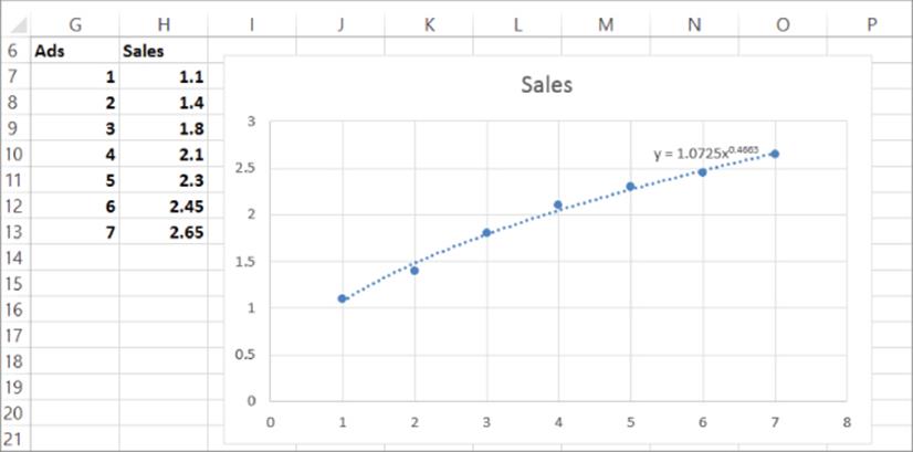
Suppose a company feels the number of units of a product sold (in thousands) in a month and the number of ads placed are related, as shown in Figure 32.1 (see Powercurve.xlsx file).
Figure 32-1: Fitting a Power curve to ad response data
To fit a Power curve to this data, complete the following steps:
1. Plot the points by selecting the range G6:H13, and from the Insert tab, select Scatter. (Choose the first option: Scatter with only markers.)
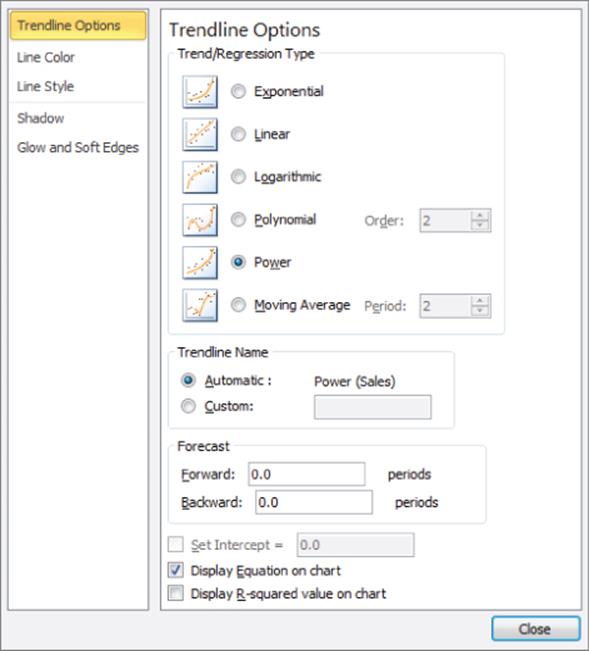
2. Right-click any point and select Add Trendline .... The Format Trendline dialog (as shown in Figure 32.2) appears.
3. Check Power and Create Equation on the chart to obtain the Power curve and equation y = 1.0725x-0.4663 shown in Figure 32.1. Note that this data (and the decreasing slope of the fitted Power curve) indicates that additional ads generate a diminishing response.
Figure 32-2: Creating the Power curve
Fitting the ADBUDG Curve
Suppose you want to determine a curve that predicts the sales of a product as a function of the sales effort allocated to the product. Researchers (see Leonard Lodish et al. “Decision Calculus Modeling at Syntex Labs,” Interfaces, 1988, pp. 5–20) have found that the response to a sales force effort can often be well described by the ADBUDG function of the following form.
![]()
Figure 32.3 shows an example of a fitted ADBUDG curve.
Figure 32-3: Fitted ADBUDG curve
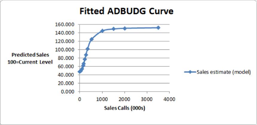
An S curve starts out flat, gets steep, and then again becomes flat. This would be the correct form of the sales as a function of effort relationship if effort needs to exceed some critical value to generate a favorable response.
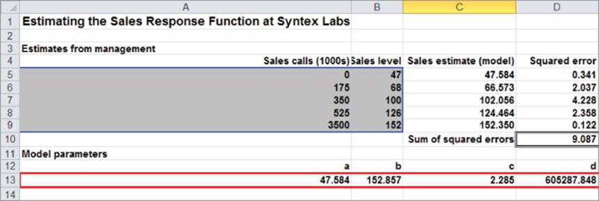
To illustrate how an ADBUDG response curve can be fit to a product, try and determine an ADBUDG curve that shows how unit sales of a drug depend on the number of sales calls made on behalf of the drug. The work for this example is in the syntexgene.xls file (see Figure 32.4).
Figure 32-4: ADBUDG curve estimation
To estimate an ADBUDG curve, use the following five points as inputs:
· Estimated sales when there is no sales effort assigned to the drug
· Estimated sales when sales effort assigned to a drug is cut in half
· Sales at current level of sales-force effort (assumed to equal a base of 100)
· Estimated sales if the sales-force effort were increased by 50 percent
· Estimated sales if the sales force “saturated” the market
Currently 350,000 calls are being made. Syntex Labs estimated that changing sales effort (refer to Figure 32.4) would have the following effects on sales:
· With no sales force effort, you can estimate sales would drop to 47 percent of their current level.
· If sales force effort were cut in half, you can estimate sales would drop to 68 percent of its current level.
· If sales force effort were increased 50 percent, you can estimate sales would increase by 26 percent.
· If you increased sales force effort 10-fold (a saturation level), you can estimate sales would increase by 52 percent.
To estimate the parameters a, b, c, and d that define the ADBUDG curve, proceed as follows:
1. Enter trial values of a, b, c, and d in A13:D13, and name these cells a, b, c, and d, respectively.
2. In cells C5:C9 compute the prediction from the ADBUDG curve by copying the formula =a+((b-a)*A5^c_)/(d+A5^c_) from C5 to C6:C9.
3. In cells D5:D9 compute the squared error for each prediction by copying the formula =(B5-C5)^2 from D5 to D6:D9.
4. In cell D10 compute the sum of the squared errors with the formula =SUM(D5:D9).
NOTE
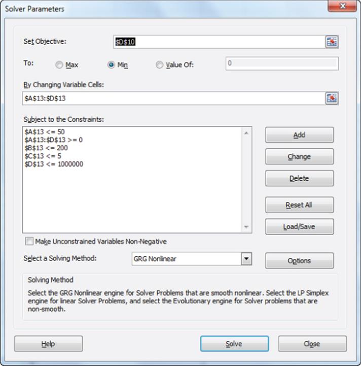
With different starting solutions the GRG Solver (without multistart) will find different final solutions. For example, if you start Solver with a = 10, b = 50, c = 5, and d = 1,000, the GRG Solver can obtain only an SSE of 3,875. With a starting solution of a = 1, b = 2, c = 3, and d = 4, you will obtain an error message! Selecting the GRG Multistart Engine ensures that your starting values of a, b, c, and d will not affect the answer found by Solver. Because a equals your predicted sales for no sales effort, a should be close to 47. (You can constrain a to be between 0 and 50.) Because b is the predicted sales with infinite sales effort, b should be close to 150. (You can constrain b to be between 0 and 200.) There are no obvious values for c and d. A large value of c, however, can cause your function to involve large numbers that may crash the GRG Multistart Engine, so constrain c to be between 0 and 5. Finally, there are no obvious limits on d, so constrain d to be between 0 and 1,000,000. The GRG multistart Solver Engine window is shown in Figure 32.5.
5. Minimize the sum of squared errors (cell D10) by changing values of a, b, c, and d (cells A13:D13). Bind a, b, c, and d as discussed previously.
Figure 32-5: Solver window for ADBUDG curve estimation
The GRG Multistart Engine found the solution shown in Figure 32.4. Observe that none of the “predictions” are off by more than 2 percent. After fitting this curve to each drug, the resulting response curves can be used as an input to a Solver model (see the next section for an example) that can determine a profit maximizing allocation of the sales force effort.
Optimizing Allocation of Sales Effort
Now that you have learned to use different types of curves to model the association between the level of marketing effort and the response, you can use this information to optimize the allocation of marketing resources. To illustrate this process, suppose you know that a Power curve can model the response to sales effort for four drugs. How would you allocate sales effort between the drugs?
In particular, suppose that units of each drug sold during a year (in thousands) are as follows:
· Drug 1 sales = 50(calls).5
· Drug 2 sales = 10(calls).75
· Drug 3 sales = 15(calls).6
· Drug 4 sales = 20(calls).3
Calls are also measured in 1,000s. For example, if 4,000 calls are made for Drug 1, then Drug 1 sales = 50(4).5 = 100,000 units. Rows 4 and 5 of the spreadsheet summarize the response curves for each drug.
In the salesallocation.xls file (see Figure 32.6), you can determine the profit, maximizing the number of sales calls made for each drug. Assume that each call costs $200 and the unit profit contribution for each drug is given in row 2.
Figure 32-6: Sales-force allocation model
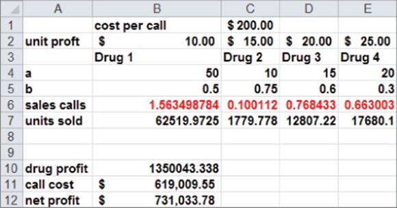
Set up the spreadsheet as follows:
1. Enter a trial number of calls for each drug in B6:E6.
2. Compute the unit sales for each drug by copying the formula =1000*B4*(B6^B5) from B7 to C7:E7.
3. In cell B10 compute the profit (excluding sales call costs) with the formula =SUMPRODUCT(B7:E7,B2:E2).
4. In cell B11 compute the annual sales call cost with the formula =1000*C1*SUM(B6:E6).
5. In cell B12 compute the net annual profit with formula =B10-B11.
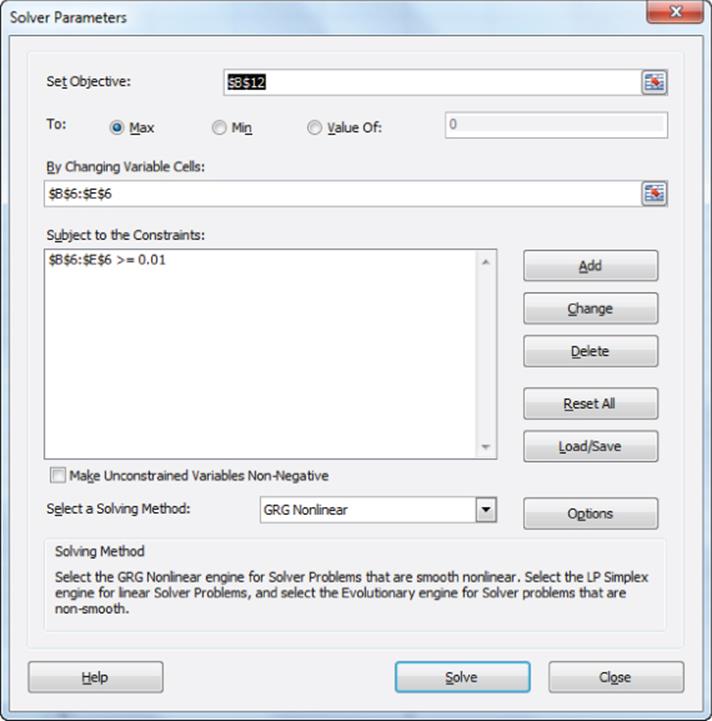
The Solver window shown in Figure 32.7 enables you to compute the profit, maximizing sales call allocation.
NOTE
Each number of calls is constrained to be >=.01 instead of 0. This prevents the Solver from trying a negative number of sales calls. If Solver tried a negative value for the calls made on behalf of a drug, then the unit sales would be undefined and would result in an error message.
Figure 32-7: Solver window for sales call allocation
A maximum profit of $731,033 is obtained with 1,562 calls for Drug 1, 100 calls for Drug 2, 769 calls for Drug 3, and 663 calls for Drug 4. As shown in Exercise 2, the Solver simply allocates the calls to each drug so that the change in the marginal profit generated by changing a drug's number of calls by a small amount (say .01) equals the cost of .01 calls. In short, the Solver finds the optimal sales force allocation by invoking the old economic adage that marginal revenue = marginal cost.
Lodish et al. (Interfaces, 1988) used the methodology of this chapter to analyze sales force allocation at Syntex Laboratories. Following their recommendations, Syntex Laboratories hired 200 more salespeople, and in just one year saw a 100-percent return on investment! Because Syntex first used these methods, Lodish et al. reported that at least 10 other pharmaceutical companies have successfully determined their sales force allocation by using the models described in this chapter.
Using the Gompertz Curve to Allocate Supermarket Shelf Space
In his paper, “Shelf Management and Space Elasticity,” Xavier Dreze et al. (see http://research.chicagobooth.edu/marketing/databases/dominicks/docs/1994-ShelfManagement.pdf) worked with Dominick's Finer Foods, a Chicago supermarket chain, to determine a profit maximizing shelf space allocation and product layout.
They first conducted a cluster analysis using customer demographic information on 60 stores. The authors decided there were two relevant clusters: urban stores and suburban stores, so they built a model for each cluster to predict sales of each brand as a function of the space allocated to the brand, brand price, and brand location (eye level, above eye level, below eye level). The relationship of a brand's sales to allocated space was modeled by a Gompertz curve, while the effect of brand price and brand location (at eye level, above eye level, or below eye level) was modeled via the SCAN*PRO model (see Exercise 6).
The authors then used Solver for a particular product category to allocate available space between brands and determine the profit-maximizing space allocation and location for each brand. The authors reported a 5 to 6 percent increase in store profits.
Summary
In this chapter you learned the following:
· The key to optimizing the allocation of marketing effort is modeling the functional relationship between the amount of effort and unit sales.
· The Power curve, ADBUDG curve, and Gompertz curve are often used to model the relationship between effort and unit sales.
· When the functional relationship between effort and unit sales is determined, a Solver model, with profit as the target cell and changing cells being the amount of effort assigned to each product, can be used to determine the allocation of marketing effort.
Exercises
1. You want to allocate 2,000 square feet of space in CVS between seasonal and nonseasonal items. You must allocate at least 400 square feet to each type of item. Estimated profit as a function of floor space is given here.
|
Space |
Seasonal Profit |
Nonseasonal Profit |
|
500 |
357,770.9 |
1,056,381.404 |
|
750 |
438,178 |
1,217,454.357 |
|
1,000 |
505,964.4 |
1,346,422.145 |
|
1,250 |
565,685.4 |
1,455,793.415 |
|
1,500 |
619,677.3 |
1,551,719.389 |
How much space should be allocated to each type of item?
2. Show in the salesallocation.xlsx file that Solver's optimal resource allocation has the property that the marginal profit generated by a small change in a drug's calls equals the sales call cost associated with the change in calls.
3. How could the ADBUDG curve be used to determine the optimal allocation of advertising dollars for GM's car models?
4. In 2009 Target began to devote a much larger portion of its stores to groceries. Why would the methods of this chapter understate the benefit Target would obtain by allocating more space to groceries?
5. Paris Lohan is a marketing analyst for Time Warner. She has fit an ADBUDG curve for each magazine that describes how the number of new subscriptions changes when the money spent on advertising the magazine changes. Paris now wants to determine a profit maximizing allocation of the ad budget for each magazine. In Paris' target cell she has multiplied the number of new subscriptions by the annual profit per subscriber to the magazine. Can you find an error in Paris' logic?
6. In Excel, set up a formula that combines the Gompertz curve and SCAN*PRO model to estimate sales of a brand as a function of brand price, brand location (eye level, above eye level, below eye level), and price of competitor's brand.
All materials on the site are licensed Creative Commons Attribution-Sharealike 3.0 Unported CC BY-SA 3.0 & GNU Free Documentation License (GFDL)
If you are the copyright holder of any material contained on our site and intend to remove it, please contact our site administrator for approval.
© 2016-2026 All site design rights belong to S.Y.A.