Marketing Analytics: Data-Driven Techniques with Microsoft Excel (2014)

Part VIII. Retailing

Chapter 33. Forecasting Sales from Few Data Points

There are many situations in which a business wants to estimate total sales of a product based on sales during the early portion of the product life cycle. This need brings forth the question, “How many months of sales are needed to make an accurate forecast of product sales during the product's lifetime?” Chapter 26, “Using S Curves to Forecast Sales of a New Product,” and Chapter 27, “The Bass Diffusion Model,” show how S curves and the Bass model can be used to predict total sales early in the product life cycle. Both the S curve and Bass model require at least five data points, however, to obtain reasonable estimates of future sales. This chapter describes a simpler method that can estimate total product sales from as few as two data points.

Predicting Movie Revenues

When a new movie comes out, how many weeks of revenue are needed to predict total movie revenue? One might guess 5 or 6, however, it is actually possible to predict a movie's total revenues from as few as 2 weeks of revenues.

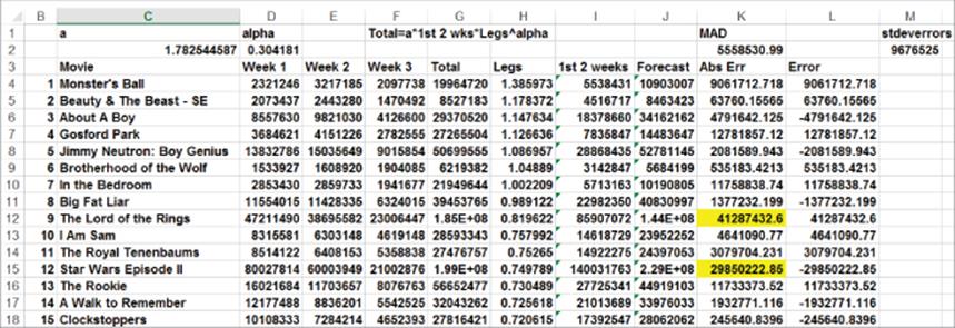
The 2weeks MAD worksheet of the finalresultmovie.xls file (see Figure 33.1) contains total revenues for 76 movies and revenues for each of the first 3 weeks of the movie's release. Using this data, the goal is to develop a simple model that can accurately predict total revenues from either the first 2 or 3 weeks of revenues. In many industries (such as video games) analysts begin with a simple rule such as the following equation:

1

Figure 33-1: Movie revenue data

For example, you may try to estimate total revenue for a movie by simply doubling the revenues earned by the movie during its first 2 weeks. To see the weakness of this type of rule though, consider the revenues (in millions of dollars) for the two movies shown in Table 33.1.

Table 33.1 Weakness of Equation 1

Because each movie made $120 million during the first 2 weeks, any prediction for total revenue generated from Equation 1 will be the same for each movie. Looking at the data tells you, however, that revenue for Movie 1 is dropping fast, but revenue for Movie 2 is holding up well. This would lead you to believe future revenue for Movie 2 will exceed Movie 1. Predicting total movie revenue with Equation 2 will create higher forecasts (after adjusting for total revenue during the first 2 weeks) for Movie 2, as wanted.

2

In Equation 2, Legs = Week 2 Revenue / Week 1 Revenue. If Legs = 1 (which is the case for Movie 2 in Table 33.1), for example, the movie has excellent staying power because Week 2 revenue = Week 1 revenue. The average value of Legs for the movies in this data set was 0.63, indicating that Week 2 revenues average 37 percent lower than Week 1 revenues. If you hold a movie's first two weeks of revenue constant, then the forecasted total revenue from Equation 2 is an increasing function of Legs, which means a movie's forecasted revenue is an increasing function of the movie's staying power.

NOTE

The term “legs” is being used as a synonym for the movie's staying power at the box office.

The worksheet 2weeks MAD uses the GRG Multistart Solver engine to determine the values of a and alpha that minimize average absolute error. Note that some movies (such as Lord of the Rings) make a lot of money relative to other movies (such as Orange County). If you minimize MAPE (Mean Absolute Percent Error), then movies that have low revenue can exert an inordinate influence on the target cell. For example, if you predicted $6 million revenue for Orange County, you were fairly close in absolute terms to the actual revenue (near $4 million) but your percentage error is nearly 50 percent.

In general, choosing SSE (Sum of Squared Error) as a goodness of fit criteria for a model causes the outliers to have a large effect on the model's estimated parameters. In contrast, if MAD (Mean Absolute Deviation) or MAPE is used as a goodness of fit criteria, then the influence of outliers on the model's estimated parameters is less and Solver concentrates on making the model fit “typical” values of the dependent variable.

To find the values of a and alpha that minimize MAD, proceed as follows:

1. Copy the formula =a*SUM(D4:E4)*(H4^alpha) from J4 to J5:J79 to generate the forecast for each movie's total revenue implied by Equation 2.

2. Copy the formula =ABS(G4-J4) from K4 to K5:K79 to compute the absolute error for each movie's prediction.

3. In cell K2 compute the average absolute error (the target cell) with the formula =AVERAGE(K4:K79).

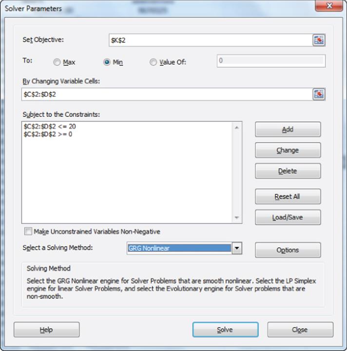
4. Using the Solver window in Figure 33.2, find values of alpha and a that minimize MAD.

Figure 33-2: Solver window for two-week movie revenue data

The resulting prediction equation is as follows:

The average error was $5.7 million. The average revenue of the listed movies is $50 million, so using 2 weeks of revenues you conclude that the forecasts are off by approximately 11 percent.

Modifying the Model to Improve Forecast Accuracy

There are a few additional measures you can take to ensure for the most accurate predictions possible. This section covers some of the most common ways you can increase the accuracy of the relatively simple model defined by Equation 2.

Finding Outliers

Recall a forecasted observation is an outlier if the absolute value of the forecast error exceeds 2 * (Standard deviation of the forecast errors). Copying the formula =G4-J4 from L4 to L5:L79 computes the forecast error for each observation. In cell M2 you can compute the standard deviation ($9.7 million) of the forecast errors with the formula =STDEV(L4:L79). Column K highlights the movie outliers, which are all movies whose forecast errors exceed 2 * 9.68 = $19.36 million. The outliers are The Lord of the Rings, Star Wars Episode II, Ocean's Eleven, Spider-Man and Monsters, Inc. If you could figure out a common thread that explained the model's lack of accuracy in predicting the revenue from these outliers, incorporating this common thread into the forecast equation would greatly improve the model's forecasting accuracy.

Minimizing Squared Errors

The 2 weeks sq error worksheet of the finalresultmovie.xls file estimates the model using the criteria of minimizing squared errors. And a = 1.84 and alpha = 0.29, which are virtually identical to the previous estimates of a and alpha. If outliers were having a large effect on the model's estimated parameters, then SSE and MAD would yield substantially different parameter estimates. The similarity of the parameter estimates for the MAD and SSE criteria shows that outliers are not having an outlandish effect on the estimates of the model's parameters.

Ignoring Staying Power

To demonstrate the improvement in forecast accuracy gained by including LEGS in the forecast model, set alpha = 0 and have Solver find the value of a that minimizes MAD (see the Simple model worksheet). The best forecast is obtained by multiplying the total revenue for the first 2 weeks by 1.53. The MAD = $6.57 million, which is 20 percent larger than the MAD obtained by including staying power in the forecast model. This calculation demonstrates the size of the benefit gained from including LEGS in the model.

Using 3 Weeks of Revenue to Forecast Movie Revenues

The preceding methods are great ways to help minimize error when you are limited to two weeks of data from which to forecast. Using three weeks of revenues, however, will clearly result in a more accurate forecast. The question is whether the additional week of data results in a substantial enough improvement in forecast accuracy. To see if it does, in the Use 3 weeks worksheet you will develop a model that forecasts total movie revenue from the first three weeks of revenue. The key issue here is how to define a movie's “staying power.” Given the first 3 weeks of a movie's revenues, you can define the following equation:

3

In Equation 3 Week 2 Legs = Week 2 Revenue / Week 1 Revenue, Week 3 Legs = Week 3 revenue / Week 2 revenue, and wt is a weight that defines the weighted average of Week 2 and Week 3 Legs that minimize MAD. The rationale behind Equation 3 is that (Week 2 Revenue / Week 1 Revenue) and (Week 3 Revenue / Week 2 Revenue) are two different estimates of a movie's staying power, so when averaged, you get a single estimate of a movie's staying power. The prediction equation is the following:

4

To find the values of a, alpha, and wt that minimize MAD, proceed as follows:

1. Copy the formula =wt*(E4/D4)+(1-wt)*(F4/E4) from H4 to H5:H79 to compute the weighted estimate of Legs for each movie.

2. Copy the formula =a*I4*(H4^alpha) from J4 to J5:J79 to compute the forecast for each movie. The absolute error and MAD formulas are as before, and the new Solver window (reflecting the fact that wt is a changing cell) is shown in Figure 33.3.

Figure 33-3: Solver window for three-week movie revenue model data

3. Use the following equation to predict Total Revenue:

The MAD has been reduced to $3.7 million.

Because most movies make most of their revenue within three weeks, it appears that including the third week in the model does not result in a substantial enough improvement in forecast accuracy to make it worth your while.

Having the ability to quickly predict future sales of a product is important in industries where demand for a new product is highly uncertain. For example, for stores that specialize in selling clothing to teens (such as PacSun and Hot Topic), ability to quickly predict future sales is vital. This is because before a new apparel item is introduced, there is great uncertainty about future product sales so a retailer can lose a lot of money if they order too much or too little. If a few weeks of data narrows the “cone of uncertainty” on future sales, then a retailer can begin with a small order and use information from a few data points to derive a reorder quantity that reduces the costs associated with overstocking or understocking the product.

Summary

In this chapter you learned the following:

· To forecast total sales of a product from the first n periods of sales, take a * (first n periods of sales) * (Legs^alpha) where Solver is used to find the values of a, alpha, and (if necessary) the parameters needed to compute Legs.

· The Target Cell can be to minimize MAD or SSE.

Exercises

1. The Newmoviedata.xlsx file contains weekly and total revenues for several movies. Develop a model to predict total movie revenues from 2 weeks of revenues.

2. For your model in Exercise 1, find all forecast outliers.

3. Think of some additional factors that could be added to the movie forecasting model that might improve forecast accuracy.

4. Suppose Microsoft asks you to determine how many weeks of sales for an Xbox game are needed to give a satisfactory forecast for total units sold. How would you proceed?

5. Why is predicting total sales of an Xbox game from several weeks of sales a more difficult problem than predicting total movie revenue from several weeks of movie revenues?