Marketing Analytics: Data-Driven Techniques with Microsoft Excel (2014)
Part IX. Advertising
Chapter 34: Measuring the Effectiveness of Advertising
Chapter 35: Media Selection Models
Chapter 36: Pay Per Click (PPC) Online Advertising
Chapter 34. Measuring the Effectiveness of Advertising
Companies have trouble measuring the effectiveness of advertising. This is due primarily to the lag between exposure to an ad and the consumer response to an ad. Simply put: past ads can (and usually do) affect present and future sales.
For example, the author taught army analysts at Fort Knox who analyzed the disposition of the Army recruiting budget. They found that many visits to Army recruiting offices could be traced to an ad that was shown on TV up to six months before.
John Wanamaker, a 19th-century Philadelphia department store merchant, summarized how difficult it is to measure the benefits of advertising when he said, “Half the money I spend on advertising is wasted; the trouble is I don't know which half.” This chapter develops several models that you can use to determine if a firm's advertising is worthwhile. You learn how to incorporate the lagged effect of advertising into your forecast of product sales. You also learn that the optimal allocation of the ad budget over time may involve either pulsing (quick bursts of intensive advertising followed by a period of no ads) or continuous spending (advertising all the time at a fairly constant rate).
The Adstock Model
Chapter 31, “Using the SCAN*PRO Model and Its Variants,” developed models that you can use to determine how price and display affect sales. These models are not too difficult to set up because you can assume that past prices and displays have no effect on current sales. However, this is not the case when it comes to advertising.
To account for the lag between exposure to an ad and the consumer response to an ad, Simon Broadbent developed the Adstock Model, detailed in his article “One Way TV Advertisements Work” (Journal of Marketing Research, 1979.) This model essentially provides a simple yet powerful way to model the fact that ads do affect present and future sales. The Adstock Model also has the virtue of being easily combined with the versions of the SCAN*PRO model discussed in Chapter 31.
The key idea behind the Adstock Model is the assumption that each given sales period or quarter you retain a fraction (lambda) of your previous stock of advertising. For example, if lambda = 0.8, then an ad from one period ago has 80 percent of the effect of an ad during the current period; an ad two periods ago has (0.80)2 = 51.2 percent as much effect as an ad during the current period; and so on. Lambda will therefore be a changing cell that is determined with Solver. In a sense the Adstock Model assumes that the effect of advertising “depreciates” or wears out in a manner similar to the way a machine wears out.
To try out an analysis using the Adstock Model, suppose you want to model sales of a seasonal price-sensitive product for which sales are trending upward. You can see in the Adstock.xlsx file that for each quarter, you are given the product price, amount of advertising, and units sold (in thousands). For example, during the first quarter of data (which was also the first quarter of the year), the price was $44.00, 44 ads were placed, and 2,639 units were sold.
Coming into the first period, you do not know the current Adstock level, so you can make the period 1 level of Adstock a changing cell (call it INITIAL ADSTOCK). Then each period's Adstock value can be computed using Equations 1 and 2:
1 ![]()
2 ![]()
Of course, you need a mechanism by which the Adstock level influences sales. You can assume that the Adstock level in a quarter has a linear effect on sales through a parameter ADEFFECT. Use the following model to forecast each quarter's sales:
3 
In Equation 3 CONST * (TRENDQuarter# + ADEFFECT * ADSTOCK) “locates” a base level for sales in the absence of seasonality and advertising and adjusts this base level based on the current Adstock level. Multiplying this base level by (PRICE)-elasticity * (Seasonal Index) adjusts the base level based on the current price and quarter of the year.
In your analysis, find the parameter values that minimize the MAPE associated with Equation 3. You could also, if desired, find the parameters that minimize SSE. The following steps describe how to use Solver to minimize MAPE.
1. In cell F6 compute quarter 1's Adstock level with the formula =E6+intialadstock*lambda using Equation 1.
2. Copy the formula =E7+lambda*F6 from F7 to F8:F29 to use Equation 2 to compute the Adstock level for the remaining quarters.
3. Copy the formula =(const*(trend)^D6+adeffect*F6)*VLOOKUP(C6,season,2)*(G6)^(-elasticity) from H6 to H7:H29 to use Equation 3 to compute a forecast for each quarter's sales.
4. Copy the formula =ABS(I6-H6)/I6 from J6 to J7:J29 to compute each quarter's absolute percentage error.
5. In cell I4 compute the MAPE with the formula =AVERAGE(J6:J29).
6. Use the Solver window in Figure 34.1 with the GRG (Generalized Reduced Gradient) Multistart engine to find the parameter values that minimize the MAPE associated with Equation 3. Most of the upper bounds on the changing cells are “intelligent guesses.” Of course, if the Solver set a changing cell value near its upper bound, you need to relax the bound. The constraint $M$11 = 1 ensures that the seasonal indices average to 1. The solution found by Solver is shown in Figure 34.2.
Figure 34-1: Solver window for Adstock Model
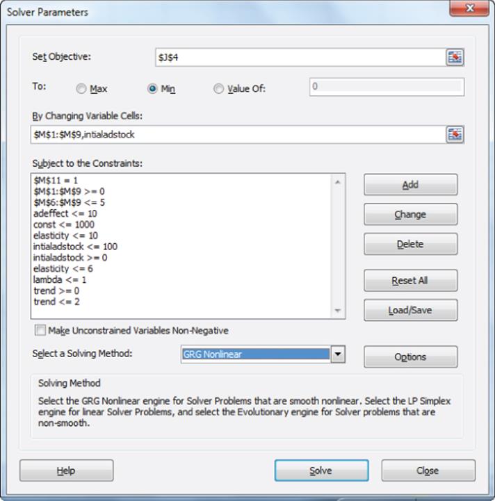
Figure 34-2: Adstock Model
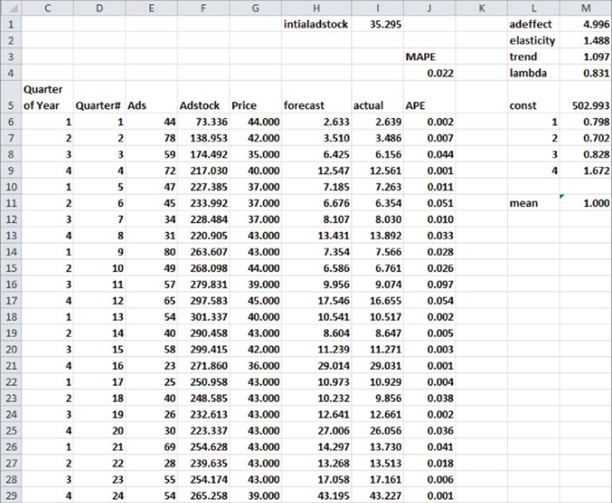
The forecasts are off by an average of 2.2 percent. The optimal values of the model parameters may be interpreted as follows:
· From cell M3 you find that sales are increasing at a rate of 9.7 percent per quarter.
· From cell M4 you find that during each quarter 17 percent (1 − 0.83) of advertising effectiveness is lost.
· From cell M2 you find that for any price a 1 percent increase in price reduces demand by 1.49 percent.
· From the values of the seasonal indices in M6:M9 you find that first quarter sales are 20 percent below sales during an average quarter; second quarter sales are 30 percent below average; third quarter sales are 18 percent below average; and fourth quarter sales are 67 percent above average. The large fourth quarter seasonality observed in this data is typical of companies (Mattel and Amazon, for example) whose sales increase greatly during the holiday season.
Another Model for Estimating Ad Effectiveness
Another model used to measure advertising effectiveness is suggested by Gary Lilien, Phillip Kotler, and Sridhar Moorthy in their book Marketing Decision Models (Prentice-Hall, 1992). The model is described by Equation 4:
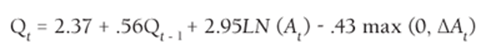
4 ![]()
In Equation 4 the following parameters are true:
· Qt = Period t sales
· At = Period t advertising
· At = Percentage increase in advertising for period t compared to period t –1
· b, c, a, and ![]() are parameters that must be estimated.
are parameters that must be estimated.
The LN (At) term incorporates the fact that the effectiveness of advertising diminishes as more advertising is done. The last term in the equation gives you an opportunity to model the effect of a change in advertising on sales. The ![]() represents the fraction of past sales used to predict current sales. Because past sales have been built up by past advertising, this term incorporates the fact that past loyalty built up through advertising affects current sales.
represents the fraction of past sales used to predict current sales. Because past sales have been built up by past advertising, this term incorporates the fact that past loyalty built up through advertising affects current sales.
In the next section you will see that the model for sales described by Equation 4 incorporates enough flexibility to enable two very different but interesting advertising strategies (pulsing and continuous spending) to be optimal in different situations.
NOTE
In contrast to the multiplicative SCAN*PRO model discussed in Chapter 31, the model defined by Equation 4 is an additive model.
You can now use this new model to measure the effectiveness of advertising based on data in the file addata.xls. This file contains 36 months of sales (in thousands of dollars) and advertising (in hundreds of dollars) for a dietary product. For variety, find the parameters defined by Equation 4that minimize SSE instead of MAPE. The following steps enable you to fit Equation 4 to this data (see Figure 34.3):
1. For each month compute At by copying from F8 to F9:F42 the formula =(D8-D7)/D7.
2. Copy the formula =a+lambda*E8+b*LN(D8)+c_*MAX(0,F8) from G8 to G9:G42 to generate the forecast for sales during months 2–36.
3. Copy the formula =(G8-C8)^2 from H8 to H9:H42 to compute the squared error for months 2–36.
4. In H5 compute SSE with the formula =SUM(H8:H42).
5. Copy the formula =C8-G8 from I8 to I9:I42 to compute the error for each month.
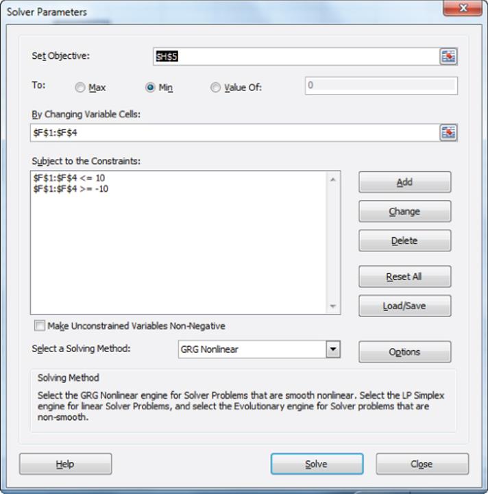
6. Use the Solver window in Figure 34.4 to estimate the parameter values.
Figure 34-3: Diet product ad data
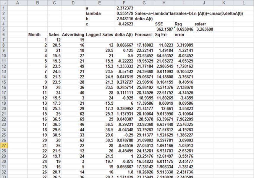
Figure 34-4: Solver window for ad data
You can find the fitted version of Equation 4 to be as follows:
The formula =RSQ(G8:G42,C8:C42) in cell I5 shows that the model explains 69 percent of sales variation. The formula =STDEV(I8:I42) in cell J5 shows that 68 percent of the forecasts should be accurate within $3,264 and 95 percent accurate within $6,528. Of course, if data were seasonal you would have to modify the model to account for the effects of seasonality as you did in the “Forecasting Software Sales” section of Chapter 31.
Optimizing Advertising: Pulsing versus Continuous Spending
Now that you have modeled the relationship between advertising and monthly sales, you may use Solver to calculate a profit-maximizing advertising strategy. The work for this example is in the optimize diet worksheet of the addata.xls file (see Figure 34.5).
Figure 34-5: Continuous spending example
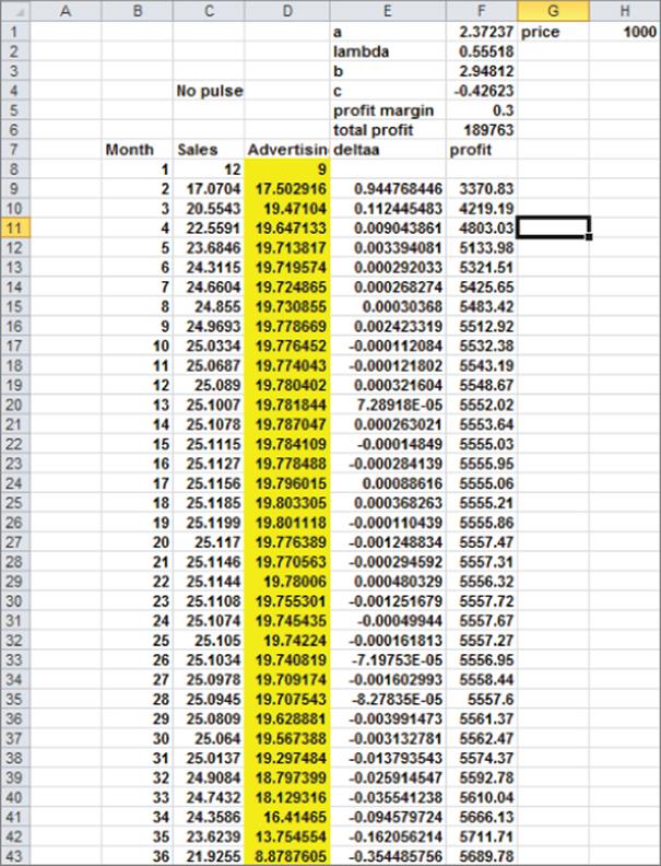
The following assumptions are made:
· 30 percent profit margin on sales
· Unit product price of $1,000
· Cost of $100 per ad
· Month 1 sales = 12 units
· Month 1 ads = 9
The goal is to use the GRG Multistart Solver engine to determine the number of ads during months 2–36 to maximize the total profit earned during months 2–36. Proceed as follows:
1. Determine the profit for months 2–36 by copying the formula =price*C9*profit_margin-100*D9 from F9 to F10:F43.
2. Generate sales in Column C during months 2–36 by copying the forecasting formula =a+lambda*C8+b*LN(D9)+c_*MAX(0,E9) from C9 to C10:C43.
The Solver window shown in Figure 34.6 determines a profit-maximizing advertising strategy:
Figure 34-6: Solver window for continuous spending example
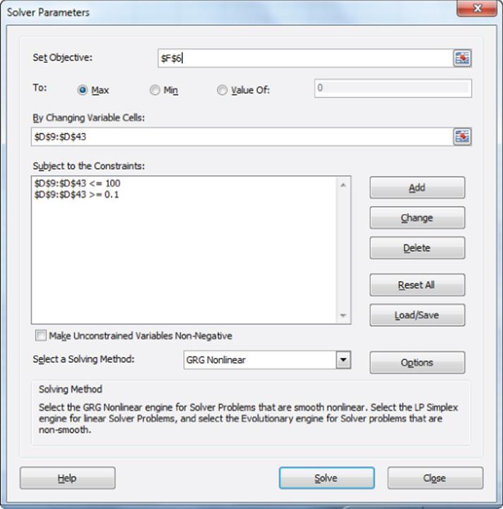
You can constrain each month's advertising to be at least .10 because an advertising level of 0 causes the LN function to be undefined, and for some reason, if you constrain a changing cell to be non-negative, Solver may try negative values for the changing cell. A relatively constant amount should be spent on advertising each month. This is known as a continuous spending strategy. During later months advertising drops because you have less of “a future” to benefit from the advertising. This is similar to the drop in retention and acquisition spending near the end of the planning horizon that was observed in Chapter 22, “Allocating Marketing Resources between Customer Acquisition and Retention.”
The pulse worksheet shows an example where several of the problem parameters are changed, and in doing so, Solver found the optimal advertising policy shown in Figure 34.7.
Figure 34-7: Example of pulsing
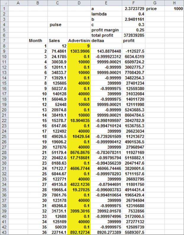
In Figure 34.7 you can observe a pulsing strategy in which you can alternate between a high and low level of advertising. Vijay Mahajan and Eitan Muller (“Advertising Pulsing Policies for Generating Awareness for New Products,” Marketing Science, 1986, pp. 89–106) discuss in more detail the conditions under which a continuous spending strategy is optimal. Prasad Naik Murali Mantrala and Alan Sawyer (“Planning Media Schedules in the Presence of Dynamic Advertising Quality,” Marketing Science, 1998, pp. 214–35) discuss conditions under which pulsing is optimal. The general consensus is that in actual situations a continuous spending strategy is much more likely to be optimal than a pulsing strategy.
Summary
In this chapter you learned the following:
· The following Adstock Model (specified by Equations 1 and 2) enables the marketing analyst to model the fact that the effect of advertising decays over time.
1 
2 
· Fitting the model shown in Equation 3 allows the marketing analyst to determine how seasonality, price, trend, and advertising affect sales.
3 
· If sales are modeled by Equation 4, then either a continuous spending or pulsing strategy can be optimal.
4 ![]()
Exercises
1. If the Adstock Model is fitted to monthly data and yields lambda = 0.7, then what would be the “half life” of advertising?
2. How could the effect of a product display on sales be incorporated into Equation 3?
3. Suppose you model daily sales of 3M painter's tape at Lowe's. 3M runs a national ad campaign for painter's tape on the Home and Garden Channel, whereas Lowe's sometimes runs ads in the local Sunday paper. How can you determine which type of advertising is more effective?
All materials on the site are licensed Creative Commons Attribution-Sharealike 3.0 Unported CC BY-SA 3.0 & GNU Free Documentation License (GFDL)
If you are the copyright holder of any material contained on our site and intend to remove it, please contact our site administrator for approval.
© 2016-2026 All site design rights belong to S.Y.A.