Marketing Analytics: Data-Driven Techniques with Microsoft Excel (2014)

Part IX. Advertising

Chapter 35. Media Selection Models

All companies that advertise must choose an allocation of their ad budgets from a large number of possible choices. These choices include allocating how much money should be spent in different ad channels such as radio, print, TV and the Internet, as well as deciding on which channels, networks, or publications each product should be advertised, and for daily shows, such as the NBC Evening News, on what days of the week the ads should be placed. To put the importance of advertising in the U.S. economy in perspective, consider that in 2013 U.S. companies spent $512 billion on advertising. The breakdown of these expenditures is as follows:

· Newspapers: $91 billion

· Magazines: $42 billion

· TV: $206 billion

· Radio: $35 billion

· Movies: $3 billion

· Outdoor: $33 billion

· Internet: $101 billion

A method used to allocate ad spending among available media vehicles that maximizes the effectiveness of the advertising is known as a media selection model. In this chapter you will learn about several widely used media selection models that can help U.S. companies allocate this $512 billion dollars more effectively.

A Linear Media Allocation Model

A.M. Lee, A.J. Burkart, Frank Bass and Robert Lonsdale were among the first researchers to use linear optimization models for media selection. Using the concepts outlined in their respective articles, “Some Optimization Problems in Advertising Media,” (Journal of the Operational Research Society, 1960) and “An Explanation of Linear Programming in Media Selection,” (Journal of Marketing Research, 1966) you can develop a linear Solver model that can be used to allocate a TV advertising budget among network TV shows to ensure that a company's ads are seen enough times by each demographic group.

Assume Honda has decided it wants its June 2014 TV ads to be seen at least this many times by the following demographic groups:

· 100 million women 18–30

· 90 million women 31–40

· 80 million women 41–50

· 70 million women more than 50

· 100 million men 18–30

· 90 million men 31–40

· 80 million men 41–50

· 70 million men more than 50

Honda can advertise on Oprah, Jeopardy!, the Late Show with David Letterman, Notre Dame Football, Saturday Night Live, The Simpsons, Seinfeld, ER, and Monday Night Football (MNF). The costs and demographic information for each show are shown in Figure 35.1, and the file Media data.xls (see the basic solver worksheet). For example, a 30-second ad on Oprah costs $32,630 and reaches 6 percent of all women 18–30, and such. There are 20 million women 18–30, and so on.

Figure 35-1: Honda's media allocation

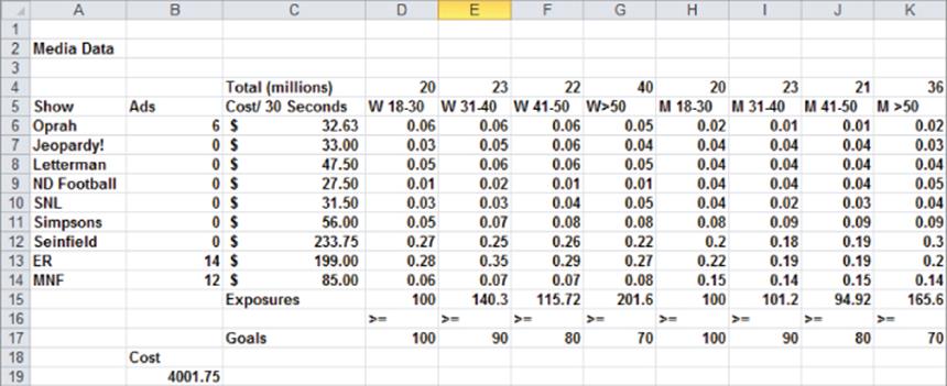
An exposure to a group occurs when a member of the group sees an ad. Honda's exposure goal for each age and gender group is given in Row 17. For example, one goal is to have your ads seen by at least 100 million women 18–30, and so on. These numbers are usually determined by either the firm's prior ad experiences or for a new product using the ad agency's prior experience.

Assuming Honda can place at most 20 ads on a given show, try and determine the cheapest way to meet its exposure goal. The following key assumptions will greatly simplify your analysis. The validity of these assumptions is discussed later in this section:

· Assumption 1: The cost of placing n ads on a show is n times the cost of placing a single ad. For example, the cost of five ads on Jeopardy! is 5 * $33,000 = $165,000.

· Assumption 2: If one ad on a show generates e exposures to a group, then n ads generates n * e exposures to a group. For example, one ad on Jeopardy! will be seen by 20 * (0.03) = 0.60 million 18–30-year-old women. This assumption implies that 10 ads on Jeopardy! would generate 10 * (0.60) = 6 million exposures to 18–30-year-old women.

· Assumption 3: The number of ads placed on each show must be an integer.

To find the cost-minimizing number of ads, proceed as follows:

1. Enter a trial number of ads on each show in range B6:B14.

2. In cell B19 compute the total cost of ads with the formula =SUMPRODUCT(B6:B14,C6:C14). This formula follows from Assumption 1.

3. Compute the total number in each demographic group seeing the ads by copying the formula =D4*SUMPRODUCT($B$6:$B$14,D6:D14) from D15 to D15:K15. This formula follows from Assumption 2.

4. The Solver window used to minimize the total cost of meeting exposure goals is shown in Figure 35.2.

Figure 35-2: Solver window for Honda's media allocation

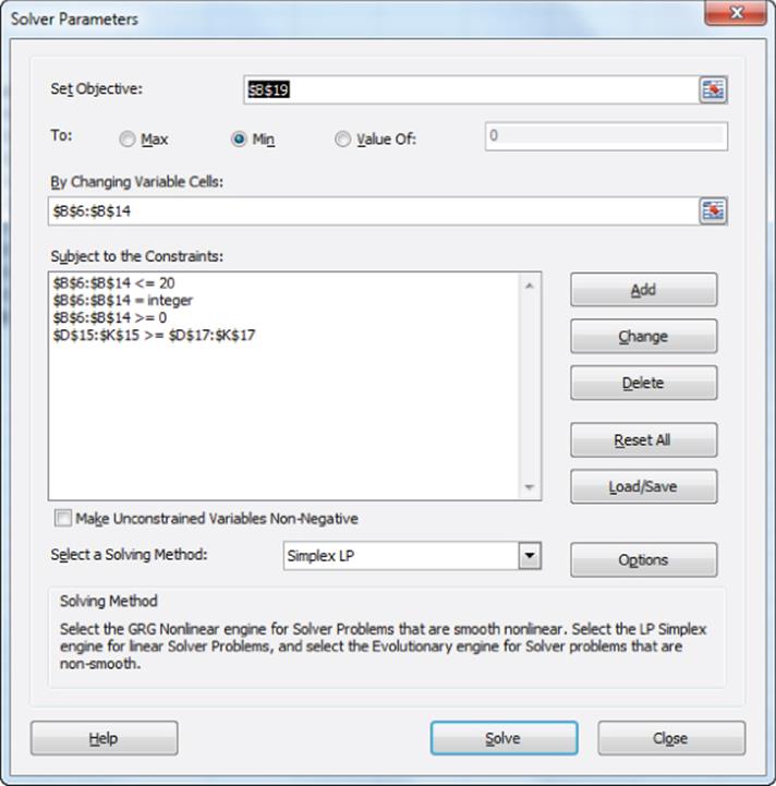
The target cell (cell B19) equals the cost of placing the ads. The changing cells (B6:B14) are the number of ads on each show. The number of ads on each show must be an integer between 0 and 20. To ensure that the ads generate the wanted number of exposures for each group, add the constraints D15:K15 >= D17:K17.

Solver finds the minimum cost is $4,001,750 and is obtained with 6 Oprah ads, 14 ER ads and 12 MNF ads.

NOTE

The assumption that the number of purchased ads must be an integer can be dropped in many cases. For example, suppose you allow the number of ads placed on a show to be fractional and Solver tells Honda to place 14.5 ads on ER. Then Honda could place 14 ads one month on ER and 15 the next month, or perhaps place 14 ads in one-half of the United States and 15 ads in the other half of the United States. If the number of ads is allowed to be a fraction then you can simply delete the integer constraints and the model will easily find a solution with possibly fractional changing cell values.

Quantity Discounts

There is a common advertising incentive that the preceding analysis doesn't take into account, however; Honda will probably receive a quantity discount if it places many ads on a given show. For example, Honda might receive a 10-percent reduction on the price of a Jeopardy! ad if it places five or more ads on Jeopardy! The presence of such quantity discounts causes the previous Solver model to be nonlinear and requires the use of Evolutionary Solver. To illustrate this, suppose that you are given the quantity discount schedule shown in Figure 35.3 (see also the QD worksheet).

Figure 35-3: Honda Quantity Discount model

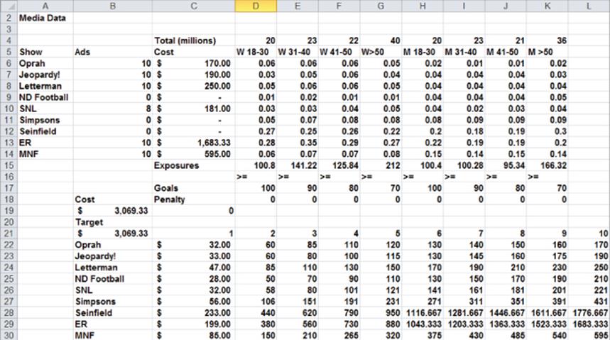
For example, 1 ad on Oprah costs $32,000, but 10 ads cost $170,000 (much less than 10 times the cost of a single ad). The goal is still to obtain the wanted number of exposures at a minimum cost. You can assume a maximum of 10 ads can be placed on each show. Recall from the discussion of the Evolutionary Solver in Chapters 5 and 6 that constraints other than bounds on changing cells (such as exposures created by ads ≥ exposures needed) should be handled using penalties. You will see that incorporating this idea is an important aspect of the model. You can proceed by using a lookup table to “look up” the ad costs and then use IF statements to evaluate the amount by which you fail to meet each goal. The target cell then minimizes the sum of costs and penalties. The work proceeds as follows:

1. Copy the formula =IF(B6=0,0,VLOOKUP(A6,lookup,B6+1,FALSE)) from C6 to C7:C14 to compute the cost of the ads on each show.

2. Copy the formula =IF(D15>D17,0,D17-D15) from D18 to E18:K18 to compute the amount by which you fall short of each exposure goal.

3. Assign a cost of 1,000 units (equivalent to $1,000,000) for each 1 million exposures by which you fail to meet a goal. Recall from Chapter 5 that the Evolutionary Solver does not handle non-linear constraints well, so you incorporate non-linear constraints by including in the target cell a large penalty for violation of a constraint.

4. In cell C19 compute the total penalties with the formula =1000*SUM(D18:K18).

5. In cell C21 add together the ad costs and constraint penalties to obtain the target cell =B19+C19.

The Solver window shown in Figure 35.4 can find the ads Honda should purchase to minimize the cost of obtaining the wanted number of exposures. The Evolutionary Solver is needed due to the use of IF statements.

Figure 35-4: Solver window for quantity discounts

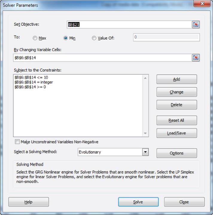
As explained in Chapters 5 and 6, the Evolutionary Solver performs better if the mutation rate is increased to 0.5. To increase the mutation rate to 0.5, select Options from the main Solver window and then choose Evolutionary Solver. Now you can adjust the mutation rate to the desired value of 0.5. A larger mutation rate reduces the change that the Solver will get stuck in a “bad” portion of the feasible region.

After setting the Solver mutation rate to 0.5, you find that the minimum cost of $3,069,000 is obtained by placing 10 ads on Oprah, Jeopardy, Letterman, ER, and MNF, and 8 ads on SNL.

A Monte Carlo Media Allocation Simulation

There are two other issues that the linear formulation model doesn't account for:

· First, Honda's goal of a wanted number of exposures for each demographic group is in all likelihood a surrogate for the wanted number of people in each group that Honda would like to see its ads. The problem with this idea is that the same person may see both an Oprah and ER ad (probably a woman) or an ER and MNF ad (probably a man). Without knowledge of the overlap or duplication between viewers of different shows, it is difficult to convert exposures into the number of people seeing a Honda ad.

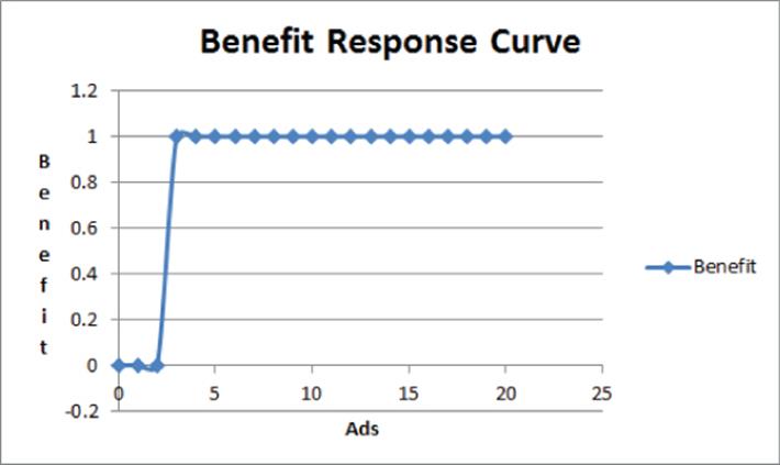
· Additionally, for any product there is a benefit-response curve that gives the benefit obtained from a person seeing any number of ads for the product. For example, in his book Marketing Analytics, (Admiral Press, 2013) Stephen Sorger states that for many products, marketers assume no benefit is obtained unless a person sees a product's ad at least three times, and additional ads do not generate any benefit to the advertiser. If this is the case, the benefit response curve for the product would look like Figure 35.5. (Chapter 32, “Allocating Retail Space and Sales Resources” discusses one method that can be used to estimate the benefit response curve.) Therefore, if Honda gains no benefit when a person sees its ad less than three times, the linear formulation does not enable Honda to determine a media allocation that minimizes the cost of obtaining a wanted benefit from the ads.

Figure 35-5: Ad response curve

To combat these issues, you can use Palisade's RISKOptimizer package (a 15-day trial version can be downloaded at www.Palisade.com) to perform a Monte Carlo simulation that will enable Honda to minimize the cost of obtaining the desired benefit from ads. In doing so, assume your goal is to have at least one-half of all people see your ads at least three times. The work for this analysis is shown in Figure 35.6 (see the ro model worksheet.)

Figure 35-6: RiskOptimizer model for media selection

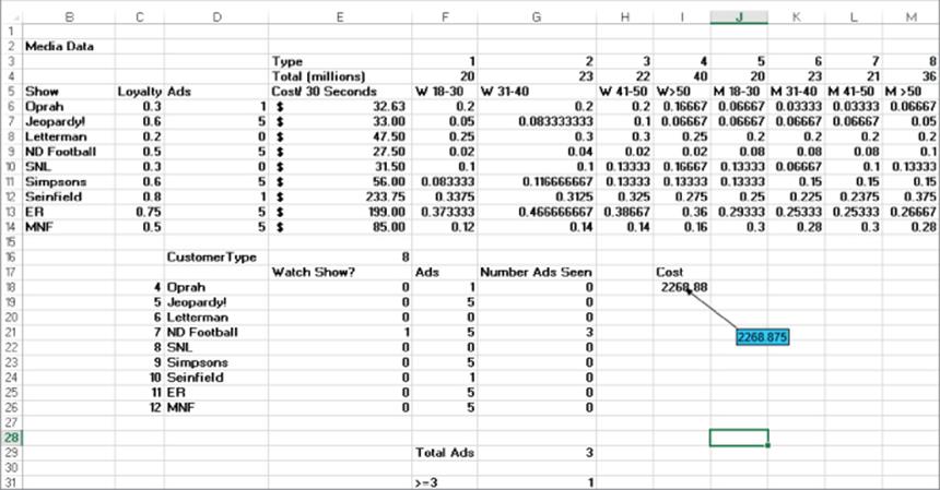
To develop this model you need to look at the demographics of each show in a different way. Referring to Figure 35.6, you can see that you are given the fraction of each group that views each show as well as the fraction of the time a viewer of a show tunes in (called loyalty). For example, 20 percent of women 18–30 are Oprah viewers, but on average an Oprah viewer watches only 30 percent of all Oprah shows. This implies, of course, that on a typical day only 6 percent of all women 18–30 watch Oprah, and this matches your previous assumption. Using this model you can randomly generate a customer and generate the number of ads seen by said customer. This approach requires some knowledge of the binomial random variable. You may recall from your statistics class that the binomial random variable is applicable in the following situation:

· Repeated trials occur with each trial resulting in a success or failure (for example, coin tosses, success = heads; shooting free throws, success = free throw is good.

· The trials are independent; that is, the outcome of any trial has no influence on the chance of success or failure on the other trials.

· Each trial has the same probability of success (0.5 on a coin toss, 0.9 if Steve Nash shoots free throws.)

The formula =RiskBinomial(n, prob) enables Palisade's RISKOptimizer add-in to generate an observation from a binomial random variable with n trials and a probability of success = prob on each trial. For example the formula =RiskBinomial(100,.5) generates the number of heads that would occur if a coin is tossed 100 times.

For any set of ads placed by Honda, you can now use RISKOptimizer to generate, say, 1,000 randomly chosen customers, and for each customer simulate the number of times the customer sees the ads. RISKOptimizer can determine if for that set of ads at least one-half of the customers see the ads at least three times. Then Evolutionary algorithms are used to adjust the number of ads to minimize the cost of the ads, subject to the constraint that at least one-half of the people see the ad at least three times. The following steps generate a random customer and her viewing patterns.

1. To begin, generate the customer type. This can be generated as a discrete random variable. For example, because there are 205 million total people, there is a 20 / 205 = 0.098 chance that a generated customer is a woman between 18 and 30.

2. For each show, determine if the generated customer sees the show by using a binomial random variable with one trial and probability of success equal to the chance that a person of the given customer type sees the show. For example, if the generated customer is a woman between 18 and 30 there is a 20-percent chance she watches Oprah.

3. Assuming the generated customer watches a show, again use a binomial random variable to determine the number of times the customer sees the ads. For example, if you placed three ads on Oprah and the generated customer was an 18–30-year-old woman, the number of times the woman sees the Oprah ads follows a binomial random variable with three trials and 0.3 chance of success.

4. In cell E16 compute a person's randomly chosen customer type with the formula =RiskDiscrete(F3:M3,F4:M4). This formula assigns a customer type from the values in the range F4:M4 with the probability of each customer type occurring being proportional to the frequencies given in the range F4:M4. Note the “probabilities” do not add up to 1, but RiskOptimizer will normalize the weights so they become probabilities. Therefore, there is a 20/205 chance the generated customer is an 18–30-year-old-woman, a 23/205 chance the generated customer is a 31–40-year-old woman, and so on.

5. Copy the formula =RiskBinomial(1,HLOOKUP($E$16,showproblook,C18,FALSE)) from E18 to E19:E26 to determine for each show if the customer is a loyal viewer. Note the customer type keys the column where you look up the probability that the customer watches the show. For the iteration shown in Figure 35.6, the simulated customer was a male >50 , so in E20 RiskOptimizer would use a 0.20 chance to determine if this customer was a Late Show viewer.

6. Copy the formula =IF(OR(E18=0,F18=0),0,RiskBinomial(F18,VLOOKUP(D18,$B$6:$C$14,2,FALSE))) from G18 to G19:G26 to simulate for each show the number of ads the viewer sees. F18 is the number of ads Honda has placed on the show. If the viewer does not view the show or 0 ads are placed, then, of course, she does not see any ads from that show. Otherwise, the lookup function in Row 18 looks up the probability that the viewer sees a particular episode of Oprah and uses the binomial random variable (number of trials = number of ads, probability of success = probability that a loyal viewer sees an ad on a show) to simulate the number of Oprah show ads seen by the viewer. For example, if E19 equals 1, the selected customer would be a male >50 Jeopardy! viewer and RiskOptimizer would use a binomial random variable with n = 5 and prob = 0.05 to simulate the number of times the simulated customer saw Jeopardy! ads.

7. In cell G29 compute the total number of ads seen by the customer with the formula =SUM(G18:G26).

8. In cell G32 give a reward of 1 if and only if a viewer saw at least three ads with the formula =IF(G29>=3,1,0).

9. In cell I18 compute the total cost of ads with the formula =SUMPRODUCT(E6:E14,D6:D14)).

You can now use the RISKOptimizer to determine the minimum cost ad strategy that ensures that at least 50 percent of all people see at least three of the ads. The RISKOptimizer window is shown in Figure 35.7.

Figure 35-7: RiskOptimizer settings for media selection

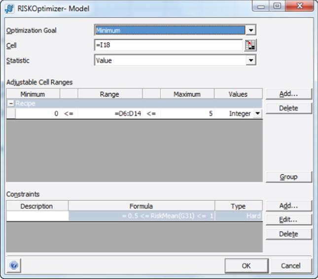
The goal is to minimize the value of the total cost (computed in I18). Assume at most five ads could be placed on each show, and you constrain the mean of G31 to be at least 0.5. This ensures that at least one-half of all people see the ads >= 3 times.

RISKOptimizer runs through different ad plans a given number of times (the example uses 1,000 iterations) and stops when it has minimized the cost of a schedule for which at least 0.5 * (1000) = 500 of the generated customers see at least three Honda ads. A minimum cost of $2,268,000 is obtained by placing the following ads:

· Five ads on Jeopardy!, Notre Dame Football, MNF, ER, and The Simpsons

· One ad on Seinfeld and Oprah

The key to the Monte Carlo media allocation approach is the fact that you can obtain for any number of n exposures the probability that a person will see your ads n times. If you know the benefit the product receives from a person seeing the ads n times you then can develop an accurate estimate of the benefit created by a product's advertising. This enables the firm or ad agency to make better media allocation decisions.

Summary

In this chapter you learned the following:

· If you assume the cost of placing n ads on a given media outlet is n times the cost of placing a single ad and n ads generates n * e exposures to a group (where e = exposures generated by one ad), then a linear Solver model can be used to generate an optimal media allocation.

· If you assume that for each customer the benefit gained from an ad depends on how many times the customer sees the ad, then the Monte Carlo simulation is needed to determine an optimal media allocation.

Exercises

1. Suppose Honda believes it obtains equal benefit from an exposure to each group. What media allocation minimizes the cost of obtaining at least 100 million exposures?

2. Suppose Honda believes the benefit from an exposure to a woman is twice the benefit from an exposure to a man. Given a budget of $5 million, where should Honda advertise?

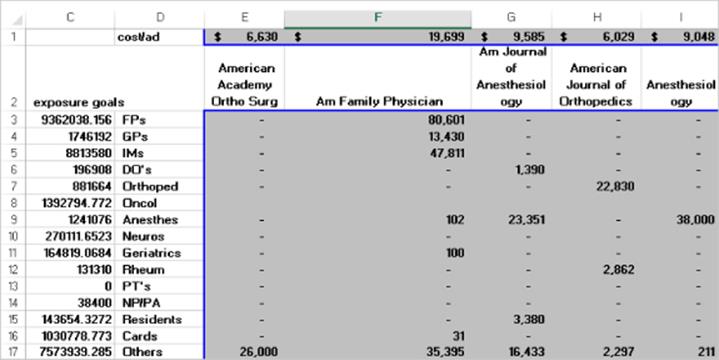
3. Drugco is trying to determine how to advertise in the leading medical journals. The Medicaldata.xlsx file (see Figure 35.8) contains the number of annual exposures to each kind of doctor Drugco wants to generate. Drugco knows the cost of a one-page ad in each journal and how many doctors of each type subscribe to each journal. For example, a one-page ad in American Family Physician (AFP) costs $19,699, and there are 80,601 family practitioners who subscribe to AFP. Assume that each journal is published 12 times a year and Drugco can place at most two ads in each issue of a journal. How can Drugco minimize the cost of obtaining the wanted number of exposures?

Figure 35-8: Medical journal data

4. Suppose Honda believes that for each demographic group the benefit obtained from any customer who sees n ads is n⁵. Given an ad budget of $5 million, what media allocation maximizes the benefits from Honda's ads?

5. How might you estimate the monetary value of the benefits Honda would gain from a TV campaign advertising a summer clearance sale?