Marketing Analytics: Data-Driven Techniques with Microsoft Excel (2014)
Part X. Marketing Research Tools
Chapter 37: Principal Component Analysis (PCA)
Chapter 38: Multidimensional Scaling (MDS)
Chapter 39: Classification Algorithms: Naive Bayes Classifier and Discriminant Analysis
Chapter 40: Analysis of Variance: One-way ANOVA
Chapter 41: Analysis of Variance: Two-way ANOVA
Chapter 37. Principal Components Analysis (PCA)
Often the marketing analyst has a data set involving many variables. For example, people might be asked to rate on a 1–5 scale the importance of 50 car characteristics, such as color, fuel economy, type of engine, and so on. Principle components analysis (PCA) is used to find a few easily interpreted variables that summarize most of the variation in the original data. As an example, this chapter describes how to use the Excel Solver to perform principal components analysis using the U.S. city demographic data that you studied in Chapter 23, “Cluster Analysis.” You'll first learn how to compute the variance of a linear combination of variables and the covariance between two linear combinations of variables, and then learn how PCA works.
Defining PCA
When you come across data sets with large amounts of variables, it can get overwhelming quickly. For instance, consider the following data sets:
· Daily returns for the last 20 years on all 30 stocks in the Dow Jones Index
· 100 measures of intelligence for a sample of 1,000 high school students
· Each athlete's score in each of the 10 events for competitors in the 2012 Olympic decathlon
These data sets contain a lot of variables, making the data difficult to understand! However, you can construct a few easily interpreted factors to help you understand the nature of the variability inherent in the original data set. For example:
· Daily stock returns might be summarized by a component reflecting the overall stock index, a component reflecting movement in the financial sector, and a component reflecting movement in the manufacturing sector.
· Intelligence might be summarized by a verbal and mathematical component.
· Ability in the decathlon might be summarized by a speed factor, a distance running factor, and a strength factor.
These factors are usually referred to as principal components; therefore an analysis of these factors is a principal component analysis, or PCA.
Linear Combinations, Variances, and Covariances
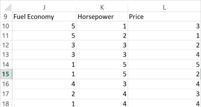
Before you can fully understand PCA, you should review some basic statistical concepts. In your review use the data in the Varcov.xlsx file (see Figure 37.1). In this file 20 people were asked to rate on a 1–5 scale (5 = highly important and 1 = not important) the role that fuel economy, engine horsepower, and price played in their purchase decision. In what follows you can assume that if you have n data points involving two variables X and Y, the data points are labeled (x1, y1), (x2, y2), … (xn, yn).
Figure 37-1: Auto attribute data
Sample Variance and Standard Deviation
The sample variance for X is defined by Equation 1:
1 
Here ![]() is the sample mean or average of the x values.
is the sample mean or average of the x values.
The sample standard deviation of X (SX) is simply the square root of the sample variance. Both the sample variance and sample standard deviation measure the spread of the variable X about its mean.
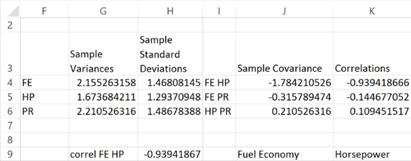
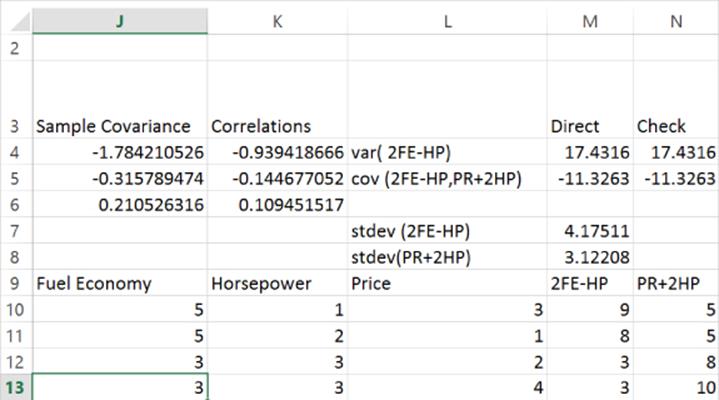
Create From Selection is used to name Columns J:L. In cell G4 (see Figure 37.2) the formula =VAR(Fuel_Economy) computes the variance (2.16) of the fuel economy ratings. Analogous formulas in G5 and G6 compute the variance for the horsepower and price ratings. In cell H4 the formula=STDEV(Fuel_Economy) computes the standard deviation (1.47) of the fuel economy ratings. Analogous formulas in H5 and H6 compute the standard deviation of the horsepower and price ratings. Of course, the standard deviation of any variable can be computed as the square root of the variance.
Figure 37-2: Sample variances and standard deviations
Sample Covariance
Given two variables X and Y, the sample covariance between X and Y, written (Sxy), is a unit-dependent measure of the linear association of X and Y. The sample covariance is computed by Equation 2:
2 
If when X is larger (or smaller) than average Y tends to be larger (or smaller) than average, then X and Y will have a positive covariance. If when X is larger (or smaller) than average Y tends to be smaller (or smaller) than average, then X and Y will have a negative covariance. In short, the sign of the covariance between X and Y will match the sign of the best-fitting line used to predict Y from X (or X from Y.) In cell J4 we computed the sample covariance (–1.78) between the FE and HP ratings with the formula =COVARIANCE.S(Fuel_Economy,Horse_Power). The .S after the word COVARIANCEensures that you divide by (n–1) and not n when computing the covariance. Analogous formulas in J5 and J6 compute the covariance between FE and PR and HP and PR.
Sample Correlations
The sample covariance is difficult to interpret because it is unit-dependent. For example, suppose that when X and Y are measured in dollars the sample covariance is $5,0002. If X and Y are measured in cents, then the sample covariance would equal 50,000,000¢2. The sample correlation (r0)) is a unit-free measure of the linear association between X and Y. The sample correlation is computed via Equation 3:
3 ![]()
The sample correlation may be interpreted as follows:
· A sample correlation near +1 means there is a strong positive linear relationship between X and Y; that is, X and Y tend to go up or down together.
· A sample correlation near –1 means there is a strong negative linear relationship between X and Y; that is, when X is larger than average, Y tends to be smaller than average, and when X is smaller than average, Y tends to be larger than average.
· A sample correlation near 0 means there is a weak linear relationship between X and Y; that is, knowledge that X is larger or smaller than average tells you little about the value of Y.
Cells K4:K6 computed the relevant sample correlations for the data. In cell K4 the formula =CORREL(Fuel_Economy,Horse_Power) computes the correlation between FE and HP (–0.94). This correlation indicates that there is a strong negative linear relationship between the importance of FE and HP in evaluating a car. In other words, a person who thinks fuel economy is important is likely not to think horsepower is important. Analogous formulas in H5 and H6 show that there is virtually no linear relationship between HP and PR or FE and PR. In short, how a person feels about the importance of price tells little about how the person feels about the importance of fuel economy and horsepower.
Standardization, Covariance, and Correlation
In the study of PCA you will be standardizing the data. Recall from Chapter 23 that a standardized value of x for the ith observation (call it zi) is defined by Equation 4.
4 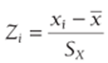
After computing the mean for each of the variables in the cell range P5:P7, you can standardize each of the variables (see Figure 37.3). For example, copying the formula =(J10-$P$5)/$H$4 from O10 to the range O11:O29 standardizes the FE ratings. You find that the first person's FE rating was 1.4 standard deviations above average. Because any standardized variable has a mean of 0 and a standard deviation of 1, standardization makes the units or magnitude of the data irrelevant.
Figure 37-3: Standardized importance ratings
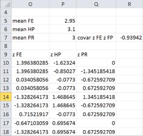
For the study of PCA, you need to know that after the data is standardized the sample covariance between any pair of standardized variables is the same as the correlation between the original variables. To illustrate this idea, use in cell R7 the formula =COVARIANCE.S(O10:O29,P10:P29) to compute the covariance between the standardized FE and HP variables. You should obtain –0.9394, which equals the correlation between FE and HP.
Matrices, Matrix Multiplication, and Matrix Transposes
A matrix is simply an array of numbers. An mxn matrix contains m rows and n columns of numbers. For example:
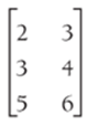 is a 2x3 matrix, [1 2] is a 1x2 matrix, and
 ![]() is a 2x1 matrix.
is a 2x1 matrix.
An mxr matrix A can be multiplied by an rxn matrix B yielding an mxn matrix whose i–j entry is obtained by multiplying the ith row of A (entry by entry) times the jth column of B. For example, if A = [1 2 3] and B = 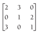 then AB = [11 5 7]. For example, the second entry in AB is computed as 1 * 3 + 2 * 1 + 3 * 0 = 5.
The transpose of an mxn matrix A is written as AT. The i–j entry in AT is the entry in row j and column i of A. For example, if A =  then AT =
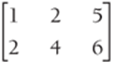
Matrix Multiplication and Transpose in Excel
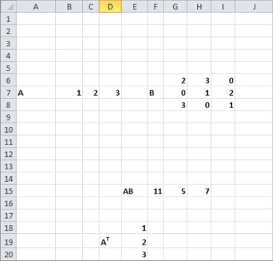
The workbook Matrixmult.xlsx shows how to multiply and transpose matrices in Excel. Matrices are multiplied in Excel using the MMULT function. MMULT is an array formula (see Chapter 3, “Using Excel Functions to Summarize Marketing Data”), so before using MMULT to multiply matrices A and B, you must select a range of cells having the same size as the product matrix AB. As shown in Figure 37.4, to compute AB complete the following steps:
1. Select the range F15:H15.
2. Array enter in cell F15 (by selecting Control+Shift+Enter) the formula =MMULT(B7:D7,G6:I8).
3. To compute AT select the range E18:E20 and array enter in cell E18 the formula =TRANSPOSE(B7:D7).
Figure 37-4: Matrix multiplication and transpose
Computing Variances and Covariances of Linear Combinations of Variables
A linear combination of n variables X1, X2, …, Xn is simply c1X1 + c2X2+ …., cnXn, where c1, c2, …., cn are arbitrary constants. Figure 37.5 shows the linear combinations 2FE - HP and PR + 2HP. For example, for the first observation 2FE − HP = 2(37.5) − 1 = 9 and PR + 2HP = 3 + (37.2)(37.1) = 5.
Figure 37-5: Computing 2FE − HP and PR + 2HP
Assuming you have n variables, you can define two linear combinations by the vectors (a vector is a matrix with one row or one column) C1 and C2.
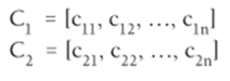
In the study of PCA you need to calculate the variance of a linear combination of the form LC1 = c11X1 + c12X2 + …., c1nXn. If you define the sample covariance matrix S for the variables X1, X2,…, Xn to be the nxn matrix whose ith diagonal entry is the sample variance of Xi and for i not equal to j, the i–jth entry of S is the sample covariance of Xi and Xj. It can be shown that the sample variance of LC1 is given by Equation 5.
5 ![]()
Here is the transpose of C1. To illustrate the use of Equation 5, compute the sample variance for 2FE-HP. In the following situation, C1 = [2 -1 0] and 
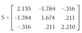
Cell N4 uses Equation 4 to compute the variance of 2FE-HP (17.43). If you array enter into cell N4 the formula =MMULT(_c1,MMULT(covar,TRANSPOSE(_c1))) you compute the variance of 2FE-HP. In cell M4 the variance of 2FE-HP is directly computed with the formula =VAR(M10:M29). Of course, the direct approach also yields a variance of 17.43.
NOTE
The range _c1 corresponds to the matrix [ 2 –1 0 ] and the range _c2 corresponds to the matrix [0 2 1].
In the study of PCA you also need to find the sample covariance between two linear combinations of variables: LC1 = c11X1 + c12X2 + …. c1nXn and LC2 = c21X1 + c22X2 + …. c2nXn. It can be shown that the following equation is true:
6 ![]()
You can illustrate the use of Equation 6 by following these steps:
1. Compute the sample covariance between 2FE - HP and PR + 2HP. Here C1 = [2 – 1 0] and C2 = [0 2 1].
2. In cell N5 compute the sample covariance between 2FE – HP and PR + 2HP (–11.236) by array entering the formula =MMULT(_c1,MMULT(covar,TRANSPOSE(_c2))).
3. In cell M5 the same result (-11.236) is obtained with the formula =COVARIANCE.S(M10:M29,N10:N29).
Diving into Principal Components Analysis
Suppose you have data involving n variables X1,X2, … Xn. Let S denote the sample covariance matrix for these variables and R denote the sample correlation matrix for these variables. Recall that R is simply the sample covariance matrix for the standardized variables. In the analysis you can determine principal components based on R, not S. This ensures that the principal components remain unchanged when the units of measurement are changed. For more detail on PCA based on the sample covariance matrix, refer to the outstanding multivariate statistics text by Richard Johnson and Dean Wichern Applied Multivariate Statistical Analysis (Prentice-Hall, 2007.)
The basic idea behind PCA is to find n linear combinations (or principal components) of the n variables that have the following properties:
· The length of each principal component (sum of the squared coefficients) is normalized to 1.
· Each pair of principal components has 0 sample covariance. Two linear combinations of variables that have 0 sample covariance are referred to as orthogonal. The orthogonality of the principal components ensures that the principal components will represent different aspects of the variability in the data.
· The sum of the variances of the principal components equals n, the number of variables. Because each of the standardized variables has a variance of 1, this means the principal components decompose the total variance of the n standardized variables. If principal components are created from a sample covariance matrix, then the sum of the variances of the principal components will equal the sum of the sample variances of the n variables.
· Given the previous restrictions, the first principal component is chosen to have the maximum possible variance. After determining the first principal component, you choose the second principal component to be the maximum variance linear combination of unit length that is orthogonal to the first principle component. You continue choosing for i = 3, …. 4, n the ith principal component to be the maximum variance linear combination that is orthogonal to the first i–1 principal components.
You can use the cluster analysis data from Chapter 23 (the clusterfactors.xlsx file) to illustrate the computation of principal components. Recall that for each of 49 U.S. cities we had the following six pieces of demographic information:
· Percentage of blacks
· Percentage of Hispanics
· Percentage of Asians
· Median age
· Unemployment rate
· Median per capita income (000s)
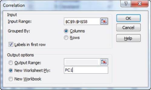
The actual data is in the cluster worksheet of workbook clusterfactors.xlsx. The sample correlations between the demographic measures will be used to perform a PCA. To obtain the sample correlations you need the Data Analysis add-in. (See Chapter 9, “Simple Linear Regression and Correlation,” for instructions on how to install the Data Analysis add-in.) To obtain the sample correlations, select Data Analysis from the Data tab, and after choosing Correlation from the Analysis dialog, fill in the dialog box, as shown in Figure 37.6.
Figure 37-6: Correlation settings for demographic data for PCA
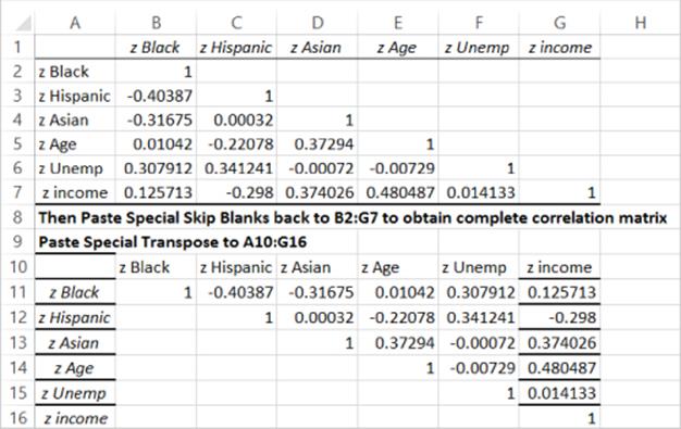
After obtaining the partial correlation matrix shown in cell range A1:G7 of Figure 37.7, select A1:G7, choose Paste Special Transpose and paste the results to the cell range A10:G16. Copy A10:G16. From the Paste Special menu, select Skip Blanks and paste back to B2:G7 to completely fill in the correlation matrix.
Figure 37-7: Filling in Correlation Matrix
Finding the First Principal Component
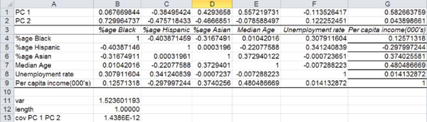
In the PC 1 worksheet (see Figure 37.8) you can find the first principal component. To do so, complete the following steps:
1. In the cell range B1:G1, enter trial values for the first principal component's weights.
2. In cell B11 compute the length of the first principal component with the formula =SUMPRODUCT(B1:G1,B1:G1).
3. Using Equation 5, the variance of the first principal component is computed in cell B10 with the array entered formula =MMULT(B1:G1,MMULT(B3:G8,TRANSPOSE(B1:G1))).
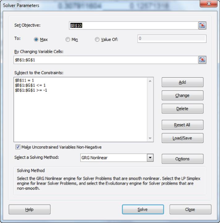
4. Use the Solver window, as shown in Figure 37.9, to determine the first principal component.
5. Maximize the variance of PC1 subject to the constraint that the length of PC1 equals 1. Use the GRG Multistart Engine, so bounds on the changing cells are required. Because the length of PC1 equals 1, each coefficient in PC must be less than 1 in absolute value, so that provides the needed bounds.
Figure 37-8: Computing first principal component
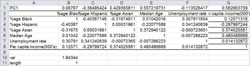
Figure 37-9: Solver window for first principal component
The goal is to pick a unit length linear combination of maximum variance. The first principal component is listed in the range B1:G1 of worksheet PC1. You find that:
![]()
The coefficient of a variable on a principal component is often referred to as the loading of the variable on the principal component. Median Age, Income, and Asian load most heavily on PC1.
PC1 explains 1.93/6 = 32 percent of the total variance in the standardized data. To interpret PC1 look at the coefficients of the standardized variables that are largest in absolute value. This shows you that PC1 can be interpreted as an older, Asian, high-income component (similar to the SF cluster from Chapter 23).
Finding the Second Principal Component
In the PC 2 worksheet you can find the second principal component (see Figure 37.10.)
Figure 37-10: Second principal component
In the cell range B2:G2 enter trial values for PC2. Then proceed as follows:
1. In cell B12 compute the length of PC2 with the formula =SUMPRODUCT(B2:G2,B2:G2).
2. In cell B11 compute the variance of PC2 by array entering the formula =MMULT(B2:G2,MMULT(B4:G9,TRANSPOSE(B2:G2))).
3. In cell B13 use Equation 6 to ensure that PC1 and PC2 have 0 covariance. Array enter the formula =MMULT(B2:G2,MMULT(B4:G9,TRANSPOSE(B1:G1))) to ensure that PC1 and PC2 have 0 covariance.
4. The Solver window shown in Figure 37.11 finds PC2.
Figure 37-11: Solver window for second principal component
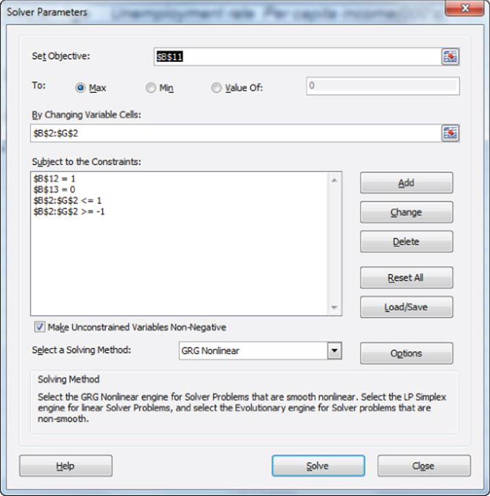
Maximize the variance of PC2 subject to the constraint that the length of PC2 = 1 and PC2 has 0 covariance with PC1. Solver tells you that PC2 is given by the following:
![]()
The first three coefficients of PC2 are large in magnitude, and the last three are small in magnitude. Ignoring the last three coefficients, you can interpret PC2 as a highly black, non-Hispanic, non-Asian factor. This corresponds to the Memphis cluster in Chapter 23. PC2 explains 1.52/6 = 25% of the variance in the data. Together PC1 and PC2 explain 32% + 25% = 57% of the variation in our data.
Each principal component will explain a lower percentage of variance than the preceding principal components. To see why this must be true, suppose the statement were not true and a principal component (say PC2 = the second principal component) explained more variation than a prior principal component (say PC1 = the first principal component). This cannot be the case because if PC2 explained more variance than PC1, Solver would have chosen PC2 before choosing PC1!
Finding PC3 through PC6
Worksheets PC 3–PC 6 compute PC3–PC6. In computing PCi (i = 3, 4, 5, 6) you can proceed as follows:
1. Copy the worksheet PCi-1 to a new worksheet. (Call it PCi.)
2. Set the coefficients for PCi as the changing cells.
3. Compute the length of PCi.
4. Compute the variance of PCi.
5. Compute the covariance of PCi with PCi-1, PCi-2, … PC1.
6. Use Solver to minimize the variance of PCi subject to a constraint that the length of PCi = 1 and all sample covariances involving the first i principal components equal 0.
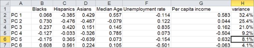
Figure 37.12 lists all six principal components, and the percentage of variance is explained by each principal component.
Figure 37-12: Final principal components
How Many Principal Components Should Be Retained?
If you have n variables, then n principal components explain all the variance in the data. The goal in performing the PCA was to explain the data with fewer than n variables. To determine the number of PCs to retain, plot the variance explained by each factor, as shown in Figure 37.13.
Figure 37-13: Variance explained by each Principal Component
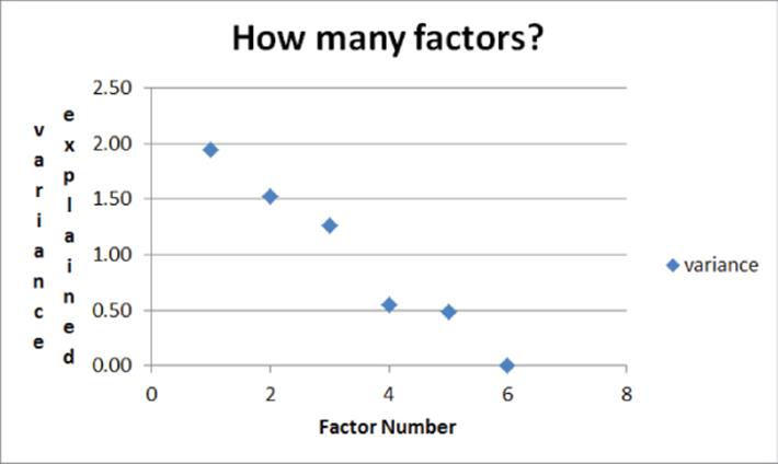
From Figure 37.13 it is clear there is a break point or elbow in the curve at the fourth PC. This indicates that after the third PC the PCs have little explanatory power, so you should keep only three factors. Note that the first three principal components explain 78 percent of the variance in the data.
In some cases there is no obvious break point. In short, the “explained variance” on the Y-axis is also referred to as an eigenvalue, and typically eigenvalues smaller than 1 indicate a principal component that explains less variance than an average principal component. For example, with six principal components the average principal component will explain a variance equaling (1/6) * 6 = 1.
Communalities
Given that you use p<n principal components (in this case p = 3), the marketing analyst would like to know what percentage of the variance in each variable is explained by the p factors. The portion of the variance of the ith variable explained by the principal components is called the ithcommunality. The ith communality is simply the sum of the squares of the loading of variable i on each of the first p components. In the Communalities worksheet (see Figure 37.14) calculate the communalities for three principal components. For example, the Communality for Percentage of Blacks if you keep the first three principal components = (0.067)2 + (0.730)2 + (0.237)2 = 59.34%.
Figure 37-14: Communalities
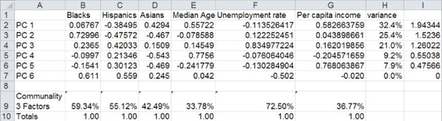
Copying from B9 to C9:G9 the formula =SUMPRODUCT(B2:B4,B2:B4) computes the six communalities. The three factors explain 72.5 percent of the variance in city unemployment rates but only 34 percent of the variance in median age. Note that most of the variance in median age is explained by PC4.
Other Applications of PCA
Donald Lehman, Sunil Gupta, and Joel Steckel (Marketing Research, Prenctice-Hall, 1997) provide an excellent application of PCA. Consumers were asked to rate on a 1–5 scale each of 10 car models on the following 15 attributes:
· Appeals to others
· Expensive looking
· Exciting
· Very reliable
· Well engineered
· Trend setting
· Has latest features
· Luxurious
· Distinctive looking
· Brand you can trust
· Conservative looking
· Family car
· Basic transportation
· High quality
Each row of data contains a consumer's 15 ratings on a given car. After using this data to compute a sample correlation matrix, a PCA was performed and the first three components explained 60 percent of the total variance. The first three factors were interpreted as the following:
· Trendy factor
· Quality and reliability factor
· Basic transportation and family friendly factor
Here you can see that PCA enables you to make sense of 15 diverse variables.
An additional application of PCA can be found in a 1988 study by A. Flood et al. from the American Journal of Clinical Nutrition that examined the eating habits of nearly 500,000 American adults. Using PCA they found three primary dietary factors:
· A fruit and vegetable factor
· A dietary food factor
· A red meat and potato factor
The authors found that people who scored high on the fruit and vegetable and dietary food factors and low on the red meat and potato factor were much less likely to get colon cancer than people who scored high on the red meat and potato factor and low on the fruit and vegetable and dietary food factors.
Summary
In this chapter you learned the following:
· You can use principal components to find a few easily interpreted variables that summarize the variation in many variables.
· This chapter assumed that all variables are standardized before the principal components are determined.
· The length of each principal component (sum of the squared coefficients) is normalized to 1.
· Each pair of principal components has 0 sample covariance. The sum of the variances of the principal components equals n, the number of variables. Because each of the standardized variables has a variance of 1, this means the principal components decompose the total variance of the n standardized variables.
· Given the previous restrictions, the first principal component is chosen to have the maximum possible variance. After determining the first principal component, you chose the second principal component to be the maximum variance linear combination of unit length that is orthogonal to the first principle component. You continued choosing for i = 3, …. 4, n the ith principal component to be the maximum variance linear combination that is orthogonal to the first i-1 principal component.
· Each principal component is interpreted by looking at the component's largest loadings.
· A plot of the variance explained by the principal components usually shows a break or elbow that indicates which principal components should be dropped.
· The communality of the ith variable is the percentage of the ith variable's variability explained by the retained principal components.
Exercises
1. The file 2012 Summer Olympics.xlsx contains for 2012 Olympic decathletes their scores on all 10 events. Use this data to determine and interpret the first three principal components.
2. The correlations between weekly returns on JPMorgan, Citibank, Wells Fargo, Royal Dutch Shell, and ExxonMobil are given in file PCstocks.xlsx. Use this data to determine and interpret the first two principal components.
3. Interpret the fourth and fifth principal components in the U.S. cities example.
4. The file cereal.xls from Chapter 23 contains calories, protein, fat, sugar, sodium, fiber, carbs, sugar, and potassium content per ounce for 43 breakfast cereals. Determine the needed principal components and interpret them.
5. The file NewMBAdata.xlsx from Chapter 23 contains average undergrad GPA, average GMAT score, percentage acceptance rate, average starting salary, and out of state tuition and fees for 54 top MBA programs. Determine the needed principal components and interpret them.
All materials on the site are licensed Creative Commons Attribution-Sharealike 3.0 Unported CC BY-SA 3.0 & GNU Free Documentation License (GFDL)
If you are the copyright holder of any material contained on our site and intend to remove it, please contact our site administrator for approval.
© 2016-2026 All site design rights belong to S.Y.A.