Marketing Analytics: Data-Driven Techniques with Microsoft Excel (2014)

Part X. Marketing Research Tools

Chapter 40. Analysis of Variance: One-way ANOVA

Often the marketing analyst wants to determine if varying a single factor has a significant effect on a marketing outcome such as sales or click-through rates. For example, take the following situations:

· Does a Valentine's Day card sell better on the top, middle, or bottom shelf?

· Does the number of click-throughs generated by an online ad depend on whether the background color is red, green, or blue?

· Do cookies sell more if they are placed on display in the candy aisle, cookie aisle, or cereal aisle?

· Does the sale of a computer book depend on whether the book is placed in the front, back, or middle of the computer section?

The factors being analyzed here include the shelf position, background color, display aisle, or placement. One-way Analysis of Variance (ANOVA) provides an easy way to help with this analysis. In this chapter you use the ANOVA: Single Factor option from the Data Analysis add-in to determine if varying a single factor such as these has a significant effect on the mean value of a marketing outcome.

Testing Whether Group Means Are Different

In one-way or single-factor ANOVA, the analyst measures the level of a response variable for G different levels of a single factor. The different levels of the single factor are often referred to as groups or treatments. For example, in the Valentine's Day example, G = 3 and the groups are the top, bottom, and middle shelf. The analyst wants to choose between the following hypotheses:

· Null Hypothesis: The means of all groups are identical. For example, in the Valentine's Day card situation, the Null Hypothesis states that mean card sales in all three shelf positions are identical.

· Alternative Hypothesis: There is a statistically significant difference between the groups' means. For example, in the Valentine's Day card situation, the Alternative Hypothesis states that there is a statistically significant difference between card sales for different shelf placement of the card.

To test these hypotheses in Microsoft Office Excel, you can use the ANOVA: Single Factor option in the Data Analysis dialog box. If the p-value computed by Excel is small (usually less than or equal to 0.05), you can conclude that the Alternative Hypothesis is true. (The means are significantly different.) If the p-value is greater than 0.05, you can conclude that the Null Hypothesis is true, that is, the group means are identical.

Example of One-way ANOVA

Suppose Wiley Publishing wants to know whether its books sell better when a display is set up in the front, back, or middle of the computer book section. Weekly sales (in hundreds) were monitored at 12 different stores. At 5 stores the books were placed in the front; at 4 stores in the back; and at 3 stores in the middle. Resulting sales are contained in the Signif worksheet in the file OnewayANOVA.xlsx, which is shown in Figure 40.1. Does the data indicate that the location of the books has a significant effect on sales?

Figure 40-1: Bookstore data where null hypothesis is rejected

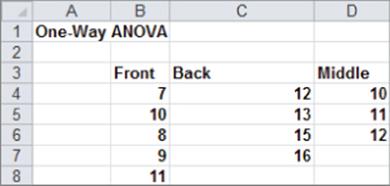
The analysis requires the assumption that the 12 stores have similar sales patterns and are approximately the same size. This assumption enables you to use one-way ANOVA because you believe that, at most, one factor (the position of the display in the computer book section) is affecting sales. (If the stores were different sizes, you would need to analyze your data with two-way ANOVA, which is discussed in Chapter 41, “Analysis of Variance: Two-way ANOVA.”)

To analyze the data, on the Data tab, click Data Analysis, and then select ANOVA: Single Factor. Fill in the dialog box, as shown in Figure 40.2.

Figure 40-2: Dialog box for bookstore example

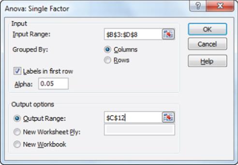
Use the following settings (The data for your input range, including labels, is in cells B3:D8.):

1. Select the Labels option because the first row of your input range contains labels.

2. Select the Columns option because the data is organized in columns.

3. Select C12 as the upper-left cell of the output range.

4. The selected Alpha value is not important. Just use the default value.

5. Click OK, and you obtain the results, as shown in Figure 40.3.

Figure 40-3: ANOVA results for bookstore example where Null Hypothesis is rejected

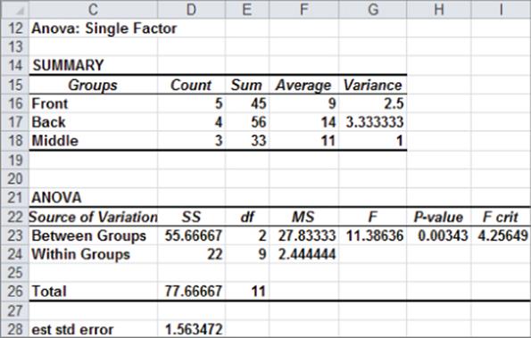
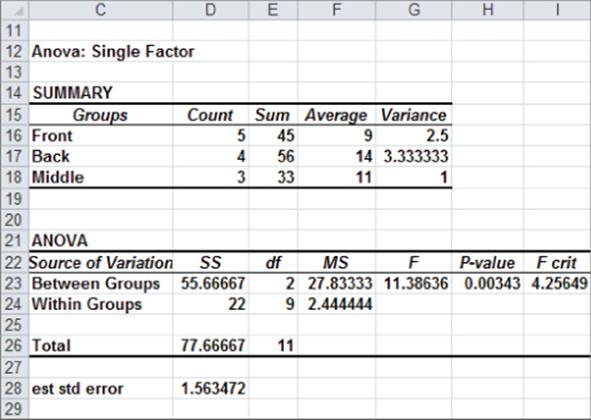
In cells F16:F18, you can see average sales depending on the location of the display. When the display is at the front of the computer book section, average sales are 900; when the display is at the back of the section, sales average 1,400; and when the display is in the middle, sales average 1,100. Because the p-value of 0.003 (in cell H23) is less than 0.05, you can conclude that these means are significantly different, so the Null Hypothesis of identical group means is rejected. Essentially the p-value of 0.003 means that if the group means were identical, there are only 3 chances in 1,000 of getting an F statistic at least as large as the observed F statistic. This small probability leads you to reject the hypothesis that the group means are identical.

The Role of Variance in ANOVA

In the Wiley bookstore example, the Null Hypothesis was rejected because the means differed significantly, but ANOVA stands for One-way Analysis of Variance, not One-way Analysis of Means. Therefore, the bookstore example result changes if you add variation in sales to your data.

Take a look instead at the data on a book sales study from the Insig worksheet of the file OnewayANOVA.xlsx, as shown in Figure 40.4. If you run a one-way ANOVA on this data, you can obtain the results shown in Figure 40.5.

Figure 40-4: Bookstore data where Null Hypothesis is accepted

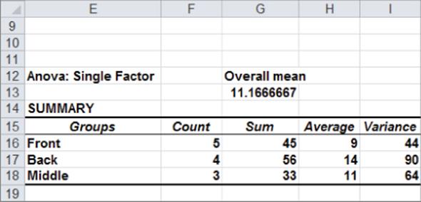
Figure 40-5: ANOVA results where Null Hypothesis is accepted

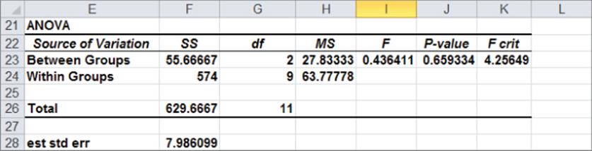
The mean sales for each part of the store are exactly as before, yet the p-value of .66 indicates that you should accept the Null Hypothesis and conclude that the position of the display in the computer book section doesn't affect sales. The reason for this strange result is that in the second data set, you have much more variation in sales when the display is at each position in the computer book section. In the first data set, for example, the variation in sales when the display is at the front is between 700 and 1,100, whereas in the second data set, the variation in sales is between 200 and 2,000. The variation of sales within each store (called the Within Groups Sum of Squares on the printout but more commonly the Sum of Squared Errors) is measured by the sum of the squares of all the observations about their group means. For example, in the first data set, the Within Groups Sum of Squares is computed as the following:

(7-9)²+(10-9)²+(8-9)²+(9-9)²+(11-9)²+(12-14)²+(13-14)²+(15-14)²+(16-14)²+(10-11)²+(11-11)²+(12-11)²=22

This measure is shown in cell D24 in the first data set and in cell F24 in the second. In the first data set, the sum of squares of data within groups is only 22, whereas in the second data set, the sum of squares within groups is 574! The large variation within the data points at each store for the second data set masks the variation between the groups (store positions) and makes it impossible to conclude for the second data set that the difference between sales in different store positions is significant. Because the variation within a group plays a critical role in determining the acceptance or rejection of the Null Hypothesis, statistics call the technique Analysis of Variance instead of Analysis of Means.

NOTE

If you simply wanted to determine the actual difference in group means (and not test for statistical significance), then you could utilize PivotTables (Chapter 1, “Slicing and Dicing Marketing Data with PivotTables”) or Excel's AVERAGEIF or AVERAGEIFS functions (Chapter 3, “Using Excel Functions to Summarize Marketing Data”).

Forecasting with One-way ANOVA

If there is a significant difference between group means, the best forecast for each group is simply the group's mean. Therefore, in the Signif worksheet in the file OnewayANOVA.xlsx, you can predict the following:

· Sales when the display is at the front of the computer book section will be 900 books per week.

· Sales when the display is at the back will be 1,400 books per week.

· Sales when the display is in the middle will be 1,100 books per week.

If there is no significant difference between the group means, the best forecast for each observation is simply the overall mean. Thus, in the second data set, you can predict weekly sales of 1,117, independent of where the books are placed.

You can also estimate the accuracy of the forecasts. The square root of the Within Groups MS (Mean Square) is the standard deviation of the forecasts from a one-way ANOVA. As shown in Figure 40.6, the standard deviation of forecasts for the first data set is 156. Two assumptions needed for a one-way ANOVA to be valid are:

· The residuals or forecast errors for each observation (residual = actual sales – predicted sales) are normally distributed.

· The variance of the residuals for each group is identical. (This is analogous to the homoscedasticity assumption for multiple regression discussed in Chapter 10.)

Figure 40-6: Computing standard deviation of forecasts

Assume that in the current example these assumptions are met. Recall that for a normal random variable, the rule of thumb tells you that for 68 percent of all observations the absolute value of the residual should be less than one standard deviation, and for 95 percent of all observations, the absolute value of the residual should be less than two standard deviations. It now follows that:

· During 68 percent of all the weeks in which books are placed at the front of the computer section, sales will be between 900–156=744 and 900+156=1056 books.

· During 95 percent of all weeks in which books are placed at the front of the computer book section, sales will be between 900–2(156)=588 books and 900+2(156)=1212 books.

Contrasts

The ANOVA output provided by Excel tells whether there is a significant difference between the group means. If a significant difference between the group means exists, then the marketing analyst often wants to dig deeper and determine which group means result in the rejection of the Null Hypothesis. The study of contrasts can help you better understand the difference between group means.

Suppose there are G groups in a one-way ANOVA and group g has an unknown mean of μg. Marketing analysts often want to analyze a quantity of the form c₁ μ₁+ c₂ μ₂+,…,c_Gμ_G, where the c_is is added to 0. Such a linear combination of the group means is called a contrast. As an example of why analyzing contrasts is important, suppose Barnes & Noble wants to determine if computer books sell at a different rate in East Coast and West Coast bookstores. During the month of June, daily sales of computer books were tracked in eight stores (see Figure 40.7 and worksheet final of workbook CityANOVA.xlsx) in each of six cities: San Francisco, Seattle, Los Angeles, New York City, Philadelphia, and Boston. Assume that all the stores are of similar size and have had similar sales patterns of books in the past. The hypothesis that East Coast and West Coast sales are the same is equivalent to Equation 1:

1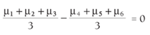

Figure 40-7: Computer book sales

The left side of Equation 1 is a contrast with c₁ = c₂ = c₃ = 1/3 and c₄ = c₅ = c₆= -1/3.

Once you have determined the contrast, you can test whether a given contrast is statistically significant from 0. For this example the following hypotheses are of interest:

· Null Hypothesis: A given contrast = 0. In this example the Null Hypothesis corresponds to average West Coast sales = average East Coast sales

· Alternative Hypothesis: The given contrast is not equal to 0. In this example the Alternative Hypothesis corresponds to average West Coast sales are not equal to average East Coast sales.

To test these hypotheses you need to compute the following test statistic:

2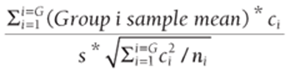

In Equation 2, n_i= number of observations taken in Group i and s = √MSE.

The p-value for the hypothesis is that the contrast =0 can be computed in Excel via the formula =T.DIST.2T(ABS(Test Statistic), N-G), where N = total number of observations. In this example N = 48 and G = 6.

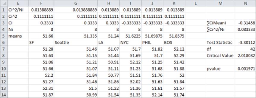
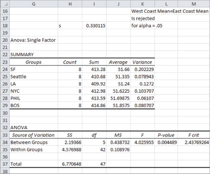
After running a one-way ANOVA on the data (refer to Figure 40.7), you obtain the results shown in Figure 40.8. Cell J35 gives the MSE = 0.108976, and you find in cell I18 that s = √0.108976 = 0.330115. The calculations to compute the test statistic are shown in Figure 40.7. Complete the following steps to test whether or not the contrast of interest is significantly different from 0.

1. In the range F3:K3 enter each C_i. The first three C_i's = 1/3 and the last three = –1/3.

2. In F4:K4 enter each N_i = 8.

3. Copy the formula =F3^2 from F2 to G2:K2 to compute each C_i^2.

4. Copy the formula =F2/F4 from F1 to G1:K1 to compute each C_i^2/N_i.

5. In cell N3 use the formula =SUMPRODUCT(F3:K3,F5:K5) to compute ∑C_i*(Sample Mean Group i).

6. In cell N4 use the formula =SUM(F1:K1) to compute ∑C_i^2/N_i.

7. In cell N6 compute the test statistic (which is known to follow a t-distribution with N – G degrees of freedom) with the formula =N3/(I18*SQRT(N4)).

8. In cell N10 compute the p-value for your hypothesis test with the formula =T.DIST.2T(ABS(N6),42). The p-value of 0.00197 indicates that according to the data, there are roughly 2 chances in 1,000 that the mean sales in East Coast and West Coast cities are identical. Therefore, you can reject the Null Hypotheses and conclude that West Coast sales of computer books are significantly higher than sales of East Coast computer books.

9. For alpha = 0.05 compute the cutoff or critical value for rejecting the Null Hypothesis in Excel with the formula =TINV(.05,N-G). In this case a test statistic exceeding 2.02 in absolute value would result in rejection of the Null Hypothesis.

Figure 40-8: ANOVA output for computer book sales

Exercise 3 will give you more practice in testing hypotheses involving contrasts.

Summary

In this chapter you learned how to analyze if a single factor has a significant effect on a measured variable.

· After running the ANOVA: Single Factor choice from Data Analysis on the Analysis group on the Data tab, you can conclude that the factor has a significant effect on the mean of the measured variable if the p-value is less than 0.05.

· If the ANOVA p-value is > 0.05, the predicted mean for each group equals the overall mean, whereas if the ANOVA p-value is < 0.05, the predicted mean for each group equals the group mean.

To test whether a contrast of the form c₁μ₁+ c₂μ₂+,…, c_gμ_g = 0, compute the test statistic using Equation 2:

2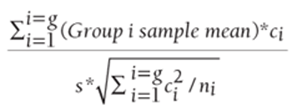

You can compute the p-value for the Null Hypothesis in Excel with the formula =T.DIST.2T(ABS(Test Statistic), N-G). If this p-value is < 0.05, the Null Hypothesis is rejected, and you conclude that the contrast is significantly different from 0. Otherwise, the Null Hypothesis is accepted.

Exercises

1. In the file Usedcars.xlsx you are given daily sales of used cars sold by four used-car salespeople.

· Is there evidence that the salespeople exhibit a significant difference in performance?

· Fill in the blank. You are 95 percent sure that the number of cars sold in a day by Salesperson 1 is between ___ and ___.

· If the first two people are men and the last two are women, is there significant evidence that the male salespeople perform differently than the female salespeople?

2. A cake can be produced by using a 400-degree, 300-degree, or 200-degree oven. In the file cakes.xlsx you are given the quality level of cakes produced when the cakes are baked at different temperatures.

· Does temperature appear to influence cake quality?

· What is the range of cake quality that you are 95 percent sure will be produced with a 200-degree oven?

· If you believe that the size of the oven used influences cake quality, does this analysis remain valid?

3. The file Salt.xlsx gives weekly sales of salt (in pounds) when one, two, and three package facings were used at Kroger's supermarkets of similar size.

· Does the number of facings impact sales of salt?

· Does adding the third facing result in a significantly different sales improvement than when adding the second facing?

4. In Exercise 3 suppose you thought there was seasonality in salt sales and the data points were from different months of the year. Could one-way ANOVA still be used to analyze the data?