Marketing Analytics: Data-Driven Techniques with Microsoft Excel (2014)

Part X. Marketing Research Tools

Chapter 41. Analysis of Variance: Two-way ANOVA

In Chapter 40, “Analysis of Variance: One-way ANOVA,” you studied one-way ANOVA where only one factor influenced a dependent variable. When two factors might influence a dependent variable, you can use two-way analysis of variance (ANOVA) to determine which, if any, of the factors have a significant influence on the dependent variable. In this chapter you learn about how two-way ANOVA can be used to analyze situations in which two factors may possibly affect a dependent variable.

Introducing Two-way ANOVA

In many marketing situations the marketing analyst believes that two factors may affect a dependent variable of interest. Here are some examples:

· How can the salespeople and their territory affect sales?

· How can price and advertising affect sales?

· How can the type of button and shape of a banner ad affect the number of click-throughs?

When two factors might influence a dependent variable you can use two-way analysis of variance (ANOVA) to easily determine which, if any, of the two factors influence the dependent variable. In two-way ANOVA the dependent variable must be observed the same number of times (call it k) for each combination of the two factors. If k = 1, the situation is called two-way ANOVA without replication. If k>1 the situation is called two-way ANOVA with replication. When k > 1 you can determine whether two factors exhibit a significant interaction (discussed in more detail in the section, “Two-way ANOVA with Interactions”). For example, suppose you want to predict sales by using product price and advertising budget. Price and advertising interact significantly if the effect of advertising depends on the product price. Interaction was discussed in the study of multiple regression in Chapter 10, “Using Multiple Regression to Forecast Sales.” In a two-way ANOVA without replication there is no way to examine the significance of interactions.

Two-way ANOVA without Replication

In a two-way ANOVA without replication you can observe each possible combination of factors exactly once. Unfortunately, there is never enough data to test for the significance of interactions. A two-way ANOVA without replication can, however, be used to determine which (if any) of two factors have a significant effect on a dependent variable.

Suppose you want to determine how a sales representative and the sales district to which the representative is assigned influence product sales. To answer the question in this example, you can have each of four sales reps spend 1 month selling in each of five sales districts. The resulting sales are given in the Randomized Blocks worksheet in the Twowayanova.xlsx file, as shown in Figure 41.1. For example, Rep 1 sold 20 units during the month she was assigned to District 4.

Figure 41-1: Randomized blocks data

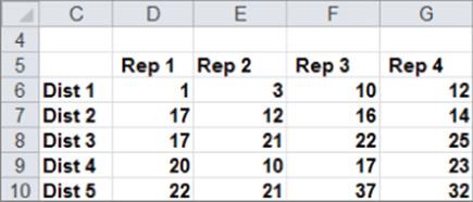
This model is called a two-way ANOVA without replication because two factors (district and sales representative) can potentially influence sales, and you have only a single instance pairing each representative with each district. This model is also referred to as a randomized block design because you can randomize (chronologically) the assignment of representatives to districts. In other words, you can ensure that the month in which Rep 1 is assigned to District 1 is equally likely to be the first, second, third, fourth, or fifth month. This randomization hopefully lessens the effect of time (a representative presumably becomes better over time) on the analysis. In a sense, you “block” the effect of districts when you try to compare sales representatives and use randomization to account for the possible impact of time on sales.

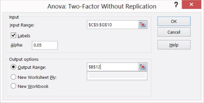
To analyze this data in Microsoft Office Excel, click Data Analysis on the Data tab, and then select the Anova: Two-Factor Without Replication option. Fill in the dialog box as shown in Figure 41.2. Use the following information to set up your analysis (the input range data is in cells C5:G10):

1. Check Labels because the first row of the input range contains labels.

2. Enter B12 as the upper-left cell of the output range.

3. The alpha value is not important, so just use the default value.

Figure 41-2: Randomized blocks dialog box settings

The output obtained is shown in Figure 41.3. (The results in cells G12:G24 were not created by the Excel Data Analysis feature. Instead, formulas are entered in these cells, as explained later in this section.)

Figure 41-3: Randomized Block output

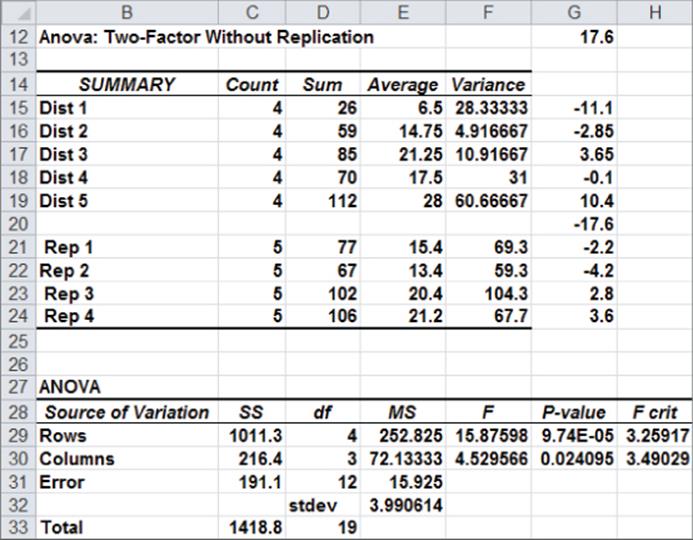
To determine whether the row factor (districts) or column factor (sales representatives) has a significant effect on sales, just look at the p-value. If the p-value for a factor is low (less than 0.05) the factor has a significant effect on sales. The row p-value (0.0000974) and column p-value (0.024) are both less than 0.05, so both the district and the representative have a significant effect on sales.

Given that the representative and the district both have significant effects on product sales, you can predict sales during a month by using Equation 1, shown here:

1

In this equation, Rep effect equals 0 if the sales rep factor is not significant. If the sales rep factor is significant, Rep effect equals the mean for the given rep minus |the overall average. Likewise, District effect equals 0 if the district factor is not significant. If the district factor is significant, District effect equals the mean for the given district minus the overall average.

In cell G12 you can compute the overall average sales (17.6) by using the formula =AVERAGE(D6:G10). The representative and district effects are computed by copying from cell G15 to G16:G24 the formula =E15–$G$12. For example, you can compute predicted sales by Rep 4 in District 2 as 17.6 – 2.85 + 3.6 = 18.35. This value is computed in cell D38 (see Figure 41.4) with the formula =G12+G16+G24. If the district effect was significant and the sales representative effect was not, the predicted sales for Rep 4 in District 2 would be 17.6 – 2.85 = 14.75. If the district was not significant and the sales rep effect was significant then the predicted sales for Rep 4 in District 2 would be 17.6 + 3.6 = 21.2.

Figure 41-4: Estimating sales by Representative 4 in District 2

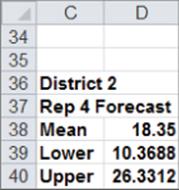
As in one-way ANOVA, the standard deviation (3.99) of the forecast errors is the square root of the mean square error shown in cell E31. This standard deviation is computed in cell E32 with the formula =SQRT(E31). Thus, you are 95 percent sure that if Rep 4 is assigned to District 2, monthly sales will be between 18.35 − 2 * (3.99) = 10.37 and 18.35 + 2 * (3.99) = 26.33. These limits are computed in cell D39 and D40 with the formulas =$D$38-2*$E$32 and =$D$38+2*$E$32, respectively.

Two-way ANOVA with Replication

When you have more than one observation for each combination of the row and column factors, you have a two-factor ANOVA with replication. To perform this sort of analysis, Excel requires that you have the same number of observations for each row-and-column combination.

In addition to testing for the significance of the row and column factors, you can also test for significant interaction between them. For example, if you want to understand how price and advertising affect sales, an interaction between price and advertising would indicate that the effect of an advertising change would depend on the price level. (Or equivalently, the effect of a price change would depend on the advertising level.) A lack of interaction between price and advertising would mean that the effect of a price change would not depend on the level of advertising.

As an example of two-factor ANOVA with replication, suppose you want to determine how the price and advertising level affects the monthly sales of a video game. In the Two Way ANOVA no interaction worksheet in the file Twowayanova.xlsx, you have the data shown in Figure 41.5. During the three months with low advertising and a medium price, for example, 21, 20, and 16 units were sold. In this example there are three replications for each price-advertising combination. The replications represent the three months during which each price-advertising combination was observed.

Figure 41-5: Data for two-way ANOVA with no interaction

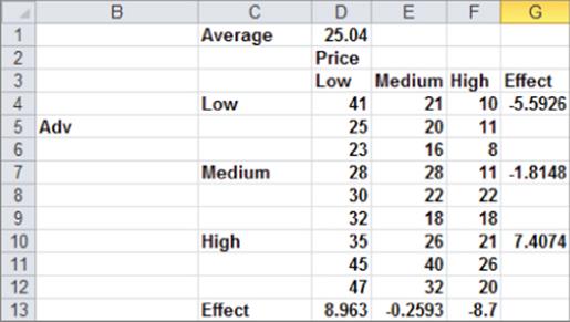
Cell D1 shows the computation for the overall average (25.037) of all observations with the formula =AVERAGE(D4:F12). Cells G4, G7, and G10, show the computation for the effect for each level of advertising. For example, the effect of having a low level of advertising equals the average for low advertising minus the overall average. Cell G4 shows the computation for the low advertising effect of –5.59 with the formula =AVERAGE(D4:F6)–$D$1. In a similar fashion, you can see the effect of each price level by copying from D13 to E13:F13 the formula =AVERAGE(D4:D12)–$D$1.

To analyze this data, click Data Analysis on the Data tab, and then select Anova: Two-Factor With Replication in the Data Analysis dialog box. Fill in the dialog box as shown in Figure 41.6.

Figure 41-6: ANOVA: Two-Factor with Replication dialog box for running a two-factor ANOVA with replication

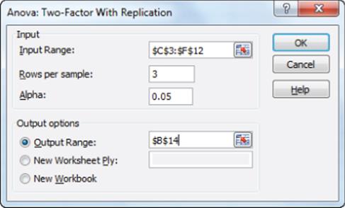
You can use the following information to set up your analysis (The input range data, including labels, is in C3:F12):

1. In two-way ANOVA with replication, Excel requires a label for each level of the column effect in the first row of each column in the input range. Thus, enter low, medium, and high in cells D3:F3 to indicate the possible price levels.

2. Excel also requires a label for each level of the row effect in the first column of the input range. These labels must appear in the row that marks the beginning of the data for each level. Thus place labels corresponding to low, medium, and high levels of advertising in cells C4, C7, and C10.

3. In the Rows Per Sample box, enter 3 because you have three replications for each combination of price and advertising level.

4. Enter B14 in the upper-left cell of the output range.

The only important portion of the output is the ANOVA table, which is shown in Figure 41.7.

Figure 41-7: Two-way ANOVA with replication output; no interaction

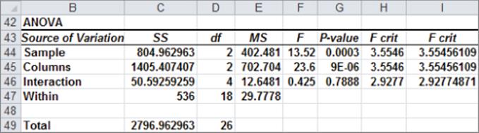
As with randomized blocks, an effect (including interactions) is significant if it has a p-value that's less than 0.05. Sample (this is the row for advertising effect) and Price (shown in the row labeled Columns) are highly significant and there is no significant interaction. (The interaction p-value is 0.79!) Therefore, you can conclude that price and advertising influence sales and that the effect of advertising on sales does not depend on the price level. Figure 41.8 graphically demonstrates that price and advertising do not exhibit a significant interaction. To create this chart, complete the following steps:

1. In the cell range I20:K22 compute the average sales for each price and advertising combination.

2. Select the range I19:K22 and select the first line chart option.

3. From the Design tab choose Switch Row/Column to place advertising categories on the x-axis.

Figure 41-8: Price and advertising do not interact in this data set

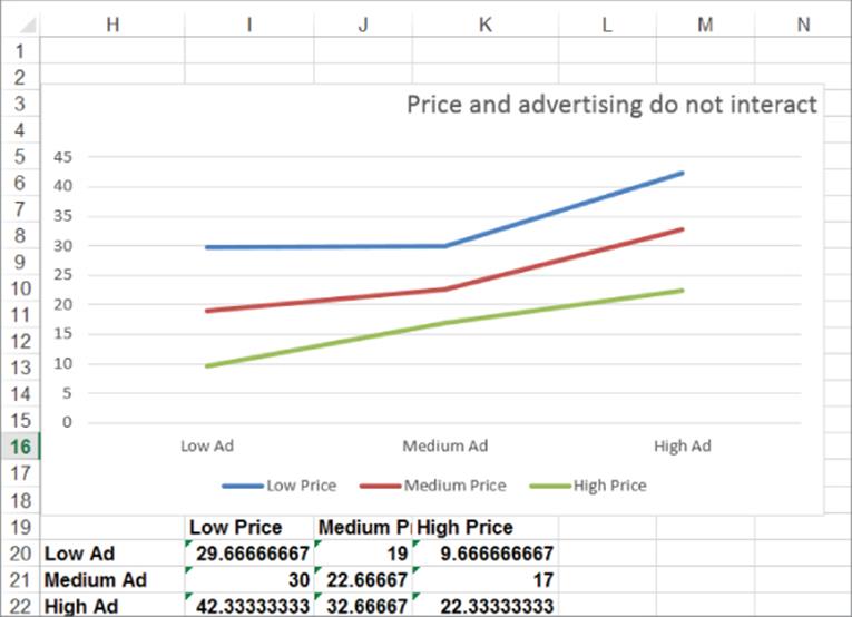
Notice that as advertising increases, sales increase at roughly the same rate, whether the price level is low, medium, or high. This fact is indicated by the near parallelism of the three curves shown in the graph.

Forecasting Sales if Interaction is Absent

In the absence of a significant interaction, you can forecast sales in a two-factor ANOVA with replication in the same way that you do in a two-factor ANOVA without replication. Use Equation 2 to do so:

2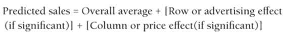

The analysis assumes that price and advertising are the only factors that affect sales. If sales are highly seasonal, seasonality would need to be incorporated into the analysis. (Seasonality was discussed in Chapters 10 and 12–14.) For example, when price is high and advertising is medium, the predicted sales are given by 25.037 + (−1.814) + (−8.704) = 14.52. (See cell E54 in Figure 41.9.) Referring to Figure 41.5, you can see that the overall average is equal to 25.037, the medium advertising effect equals –1.814, and the high price effect equals –8.704.

Figure 41-9: Forecast for sales with high price and medium advertising

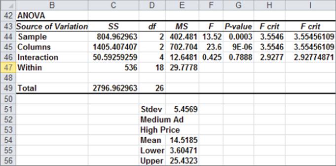
The standard deviation of the forecast errors equals the square root of the mean squared within error. For this example the standard deviation of the forecast errors is given by √29.78 = 5.46.

You are 95 percent sure that the forecast is accurate within 10.92 units. In other words, you are 95-percent sure that sales during a month with high price and medium advertising will be between 3.60 and 25.43 units. This interval is very wide, suggesting that even after knowing the price and advertising level, a great deal of uncertainty remains about the level of sales.

Two-way ANOVA with Interactions

The Two WAY ANOVA with Interaction worksheet contains data from the previous example changed to the data shown in Figure 41.10. After running the analysis for a two-factor ANOVA with replication, you can obtain the results shown in Figure 41.11.

Figure 41-10: Sales data with interaction between price and advertising

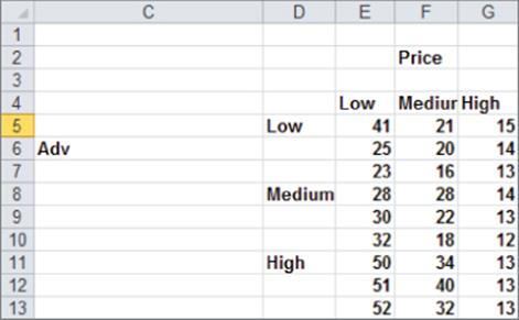
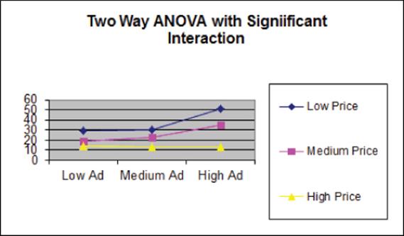
Figure 41-11: Output for the two-way ANOVA with Interaction

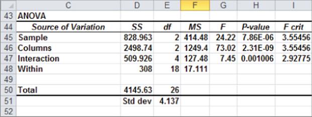
In this data set, you can find the p-value for interaction is 0.001. When you see a low p-value (less than 0.05) for interaction, do not even check p-values for row and column factors! You simply forecast sales for any price and advertising combination to equal the mean of the three observations involving that price and advertising combination. For example, the best forecast for sales during a month with high advertising and medium price is:

The standard deviation of the forecast errors is again the square root of the mean square within = 4.137 units

Thus you are 95-percent sure that the sales forecast is accurate within 8.27 units.

Figure 41.12 illustrates why this data exhibits a significant interaction between price and advertising. For a low and medium price, increased advertising increases sales, but if price is high, increased advertising has no effect on sales. This explains why you cannot use Equation 2 to forecast sales when a significant interaction is present. After all, how can you talk about an advertising effect when the effect of advertising depends on the price? Figure 41.12 is in sharp contrast to Figure 41.8 in which the near parallelism of the three curves indicates that for any level of price a change in advertising has a similar effect.

Figure 41-12: Price and advertising exhibit significant interactions in this set of data

Summary

In this chapter you learned the following:

· For two-way ANOVA without replication a factor is significant if its p-value is less than 0.05.

· For two-way ANOVA without replication the predicted value of the response variable is computed from Equation 1:

1

· In Equation 1 a factor effect is assumed to equal 0 if the factor is not significant.

· For two-way ANOVA with replication, first check if the Interaction effect is significant. This occurs if the p-value is less than 0.05. If the interaction effect is significant, then predict the value of the response variable for any combination of factor values to equal the mean of all observations having that combination of factor levels.

· If the interaction effect is not significant, then the analysis proceeds as in the two-way ANOVA without replication case.

Exercises

1. Assume that pressure (high, medium, or low) and temperature (high, medium, or low) influence the yield of a production process. Given this theory, use the data in the file Yield.xlsx to determine the answers to the following:

(a) Use the data in file Yield.xlsx to determine how temperature and/or pressure influence the yield of the process.

(b) With high pressure and low temperature, you are 95-percent sure that the process yield will be in what range?

2. Determine how the particular sales representative and the number of sales calls (one, three, or five) made to a doctor influence the amount (in thousands of dollars) that each doctor prescribes of a drug. Use the data in the Doctors.xlsx file to determine the answers to the following problems:

(a) How can the representative and number of sales calls influence the sales volume?

(b) If Rep 3 makes five sales calls to a doctor, you are 95-percent sure she will generate prescriptions within what range of dollars?

3. Answer the questions in Exercise 2 using the data in the Doctors2.xlsx workbook.

4. The Coupondata.xlsx file contains information on sales of peanut butter for weeks when a coupon was given out (or not) and when advertising was done (or not) in the Sunday paper. Describe how the coupon and advertising influence peanut butter sales.