Marketing Analytics: Data-Driven Techniques with Microsoft Excel (2014)
Part II. Pricing
Chapter 6. Nonlinear Pricing
Nonlinear pricing is used in a situation in which the cost of purchasing q units is not equal to the unit cost c per unit times q. Bundling (discussed in Chapter 5, “Price Bundling”) is a special type of nonlinear pricing because the price of three items is not equal to the sum of the individual prices.
Other common examples of nonlinear pricing strategies include:
· Quantity discounts: If customers buy ≤CUT units, they pay high price (HP) per unit, and if they buy >CUT units, they pay low price (LP) per unit. CUT is simply the “cutoff point at which the charged price changes.” For example, if customers buy ≤1000 units, you charge $10 a unit, but if they buy more than 1000 units, you charge $8 per unit for all units bought. This form of nonlinear pricing is called the nonstandard quantity discount. Another type of quantity discount strategy is as follows: Charge HP for the first CUT units bought, and charge LP for remaining units bought. For example, you charge $10 per unit for first 1000 units and $8 per unit for remaining units bought. This form of nonlinear pricing is called the standard quantity discount. In both examples the value of CUT = 1000.
· Two-part tariff: The cost of buying q units is a fixed charge K plus $c per unit purchased. For example, it may cost $500 to join a golf club and $30 per round of golf.
Many companies use quantity discounts and two-part tariffs. Microsoft does not charge twice as much for 200 units, for example, as for 100 units. Supermarkets charge less per ounce for a 2-pound jar of peanut butter as for a 1-pound jar of peanut butter. Golf courses often use a two-part tariff by charging an annual membership fee and a charge for each round of golf.
Just as in Chapter 5 you used the Evolutionary Solver to find optimal price bundling strategies, you can use the Evolutionary Solver to find the profit maximizing parameters of a nonlinear pricing strategy. As in Chapter 5, you can assume the consumer will choose an option giving her the maximum (non-negative) consumer surplus. You can see that nonlinear pricing can often significantly increase your profits, seemingly creating profits out of nothing at all.
In this chapter you will first learn how a consumer's demand curve yields the consumer's willingness to pay for each unit of a product. Using this information you will learn how to use the Evolutionary Solver to determine profit or revenue maximizing nonlinear pricing strategies.
Demand Curves and Willingness to Pay
A demand curve tells you for each possible price how many units a customer is willing to buy. A consumer's willingness to pay curve is defined as the maximum amount a customer is willing to pay for each unit of the product. In this section you will learn how to extract the willingness to pay curve from a demand curve.
Suppose you want to sell a software program to a Fortune 500 company. Let q equal the number of copies of the program the company demands, and let p equal the price charged for the software. Suppose you estimated that the demand curve for software is given by q = 400 – p. Clearly, your customer is willing to pay less for each additional unit of your software program. Locked inside this demand curve is information about how much the company is willing to pay for each unit of your program. This information is crucial to maximize profitability of sales.
Now rewrite your demand curve as p = 400 – q. Thus, when q = 1, p = $399, and so on. Now try to figure out the value your customer attaches to each of the first two units of your program. Assuming that the customer is rational, the customer will buy a unit if and only if the value of the unit exceeds your price. At a price of $400, demand equals 0, so the first unit cannot be worth $400. At a price of $399, however, demand equals 1 unit. Therefore, the first unit must be worth somewhere between $399 and $400. Similarly, at a price of $399, the customer does not purchase the second unit. At a price of $398, however, the customer is purchasing two units, so the customer does purchase the second unit. Therefore, the customer values the second unit somewhere between $399 and $398. The customer's willingness to pay for a unit of a product is often referred to as the unit'sreservation price.
It can be shown that a good approximation to the value of the ith unit purchased by the customer is the price that makes demand equal to i –0.5. For example, by setting q equal to 0.5, you can find that the value of the first unit is 400 –0.5 = $399.50. Similarly, by setting q = 1.5, you can find that the value of the second unit is 400 – 1.5 = $398.50.
Suppose the demand curve can be written as p = D(q). In your example this looks like D(q) = 400 –q. The reader who knows integral calculus can exactly determine the value a consumer places on the first n items by computing ∫n0D(q)dq. In your example you would find the value of the first two units to be the following:
![]()
This agrees with your approximate method that yields a value of 399.5 + 398.5 = 798 for the first two units.
Profit Maximizing with Nonlinear Pricing Strategies
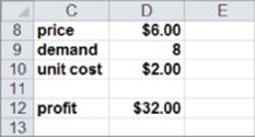
Throughout this chapter assume a power company (Atlantis Power and Light, APL for short) wants to determine how to maximize the profit earned from a customer whose demand in kilowatt hours (kwh) for power is given by q = 20 – 2p. It costs $2 to produce a unit of power. Your analysis begins by assuming APL will use linear pricing; that is, charging the same price for each unit sold. You will find that with linear pricing the maximum profit that can be obtained is $32. Then you will find the surprising result that proper use of quantity discounts or a two-part tariff doubles APL's profit! The work for this chapter is in the file Powerblockprice.xls. To determine the profit maximizing linear pricing rule, you simply want to maximize (20 – 2p) × (p – 2). In the oneprice worksheet from the Powerblockprice.xls file, a price of $6 yields a maximum profit of $32 (see Figure 6.1). The Solver model simply chooses a non-negative price (changing the cell that maximizes profit [Cell D12]). Charging $6 per kwh yields a maximum profit of $32.00.
Figure 6-1: Finding the profit maximizing single price strategy
Optimizing the Standard Quantity Discount
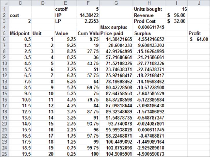
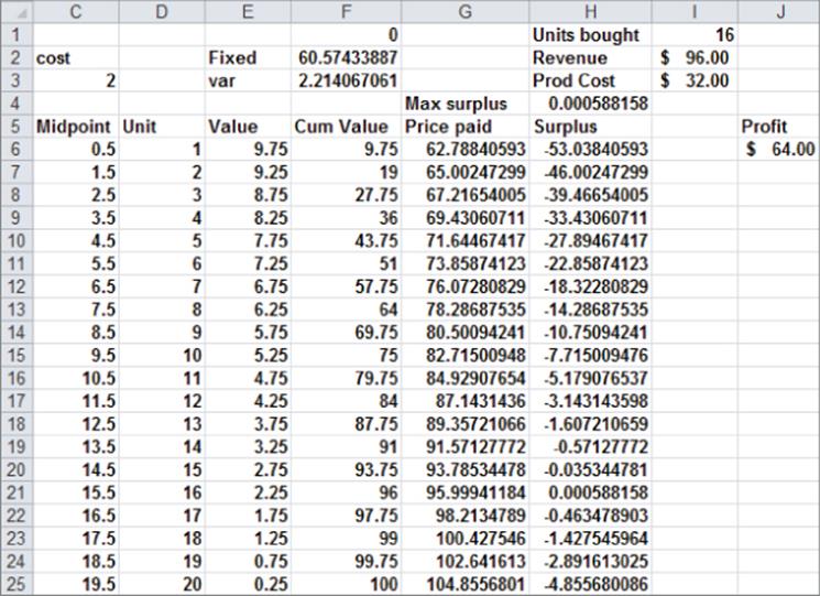
To determine a profit maximizing pricing strategy that uses the standard quantity discount, assume the quantity discount pricing policy is defined as follows: All units up to a value CUT are sold at a high price (HP). Recall that CUT is simply the cutoff point at which the per unit price is lowered. All other units sell at a lower price (LP). Assuming the customer chooses the number of kwh with the highest non-negative surplus, you can use the Evolutionary Solver to determine profit maximizing values of CUT, HP, and LP. The work for this task is shown in sheet qd of filePowerblockprice.xls. Also, Figure 6.2 shows that the demand curve may be written as p = 10 – (q/2), so the first unit is valued at 10 – (.5/2) = $9.75, the second unit is valued at 10 – (1.5/2) = $9.25, and so on.
Figure 6-2: Finding the profit maximizing standard quantity discount strategy
To complete the determination of the profit maximizing standard quantity discount strategy, complete the following steps:
1. Copy the formula =10-0.5*C6 from E6 to E7:E25 to determine the value of each unit.
2. In column F compute the cumulative value associated with buying 1, 2,…19 units. In F6 compute the value of the first unit with formula =E6. Copy the formula =F6+E7 from F7 to F8:F25 to compute the cumulative value of buying 2, 3,…20 units.
3. Copy the formula =IF(D6<=cutoff,HP*D6,HP*cutoff+LP*(D6-cutoff)) from G6 to G7:G25 to compute the total cost the consumer pays for purchasing each number of units. If you want to analyze different nonlinear pricing strategies, just change this column to a formula that computes the price the customer is charged for each number of units purchased.
4. Copy the formula =F6-G6 from H6 to H7:H25 to compute the consumer surplus associated with each purchase quantity. In cell H4 compute the maximum surplus with the formula =IF(MAX(H6:H25)>= 0,MAX(H6:H25),0); if it is negative no units will be bought, and in this case you enter a surplus of 0.
5. In cell I1 use the match function to compute the number of units bought with the function =IF(H4>0,MATCH(H4,H6:H25,0),0).
6. In cell I2 compute the sales revenue with the formula =IF(I1=0,0,VLOOKUP(I1,lookup,4)). The range D5:G25 is named Lookup.
7. In cell I3 compute production cost with the formula =I1*C3.
8. In cell J6 compute profit with the formula =I2-I3.
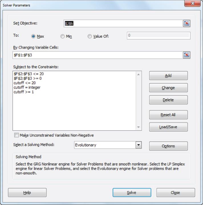
9. Use Solver to find the values of CUT, HP, and LP that maximize profit. The Solver window is shown in Figure 6.3.
Figure 6-3: Determining the profit maximizing standard quantity discount
You can constrain the value of CUT and each price to be at most $20. To do so, charge $14.30 per unit for the first 5 units and $2.22 for remaining units. A total profit of $64 is earned. The quantity discount pricing structure here is an incentive for the customer to purchase 16 units, whereas linear pricing results in the customer purchasing only 6 units. After all, how can the customer stop at 6 units when later units are so inexpensive?
Optimizing the Nonstandard Quantity Discounts
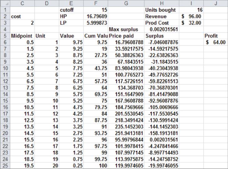
Now assume that your quantity discount strategy is to charge a high price (HP) if at most CUT units are purchased, and if more than CUT units are purchased, all units are sold at a low price (LP). The only change needed to solve for the profit maximizing strategy of this form (see sheet qd2) is to copy the formula =IF(D6<=cutoff,HP*D6,LP*D6) from G6 to G7:G25. Then just rerun the Solver window, as shown in Figure 6.3. This pricing strategy, shown in Figure 6.4, maximizes the profit: If the customer buys up to 15 units, he pays $16.79, and if he buys at least 16 units, he pays $6 per unit. Then the customer buys 16 units, and you make $64 in profit.
Figure 6-4: profit maximizing nonstandard quantity discount
Optimizing a Two-Part Tariff
Organizations such as a golf country club or Sam's Club find it convenient to give the consumer an incentive to purchase many units of a product by charging a fixed fee to purchase any number of units combined with a low constant per unit cost. This method of nonlinear pricing is called a two-part tariff. To justify paying the fixed fee the customer needs to buy many units. Of course, the customer will not buy any units whose unit cost exceeds the consumer's reservation price, so the organization must be careful to not charge a unit price that is too high.
For example, when you join a country club, you often pay a fixed fee for joining and then a constant fee per round of golf. You might pay a $500 per year fixed fee to be a club member and also pay $30 per round of golf. Therefore one round of golf would cost $530 and two rounds of golf would cost $560. If a two-part tariff were linear then for any number of purchased units, the cost per unit would be the same, but because one round cost $530 per round and two rounds costs $530/2 = $265, the two-part tariff is not consistent with linear pricing.
To dig a little deeper into the concept of a two-part tariff, look at the worksheet tpt. You will see how a power company can optimize a two-part tariff by performing the following steps:
1. To begin, make a copy of your QD or QD2 worksheet.
2. In F2 enter a trial value for the fixed fee, and in F3 enter a trial value for the price per unit. Name cell F2 Fixed and cell F3 var. The only formulas that you need to change are the formulas in the Price Paid formula in Column G (see Figure 6.5).
Figure 6-5: Optimizing a two-part tariff
3. Copy the formula =Fixed+D6*Var from G6 to G7:G25, to compute the cost of buying each number of units.
4. Adjust the Solver window, as shown in Figure 6.6.
Figure 6-6: Solver window for two-part tariff
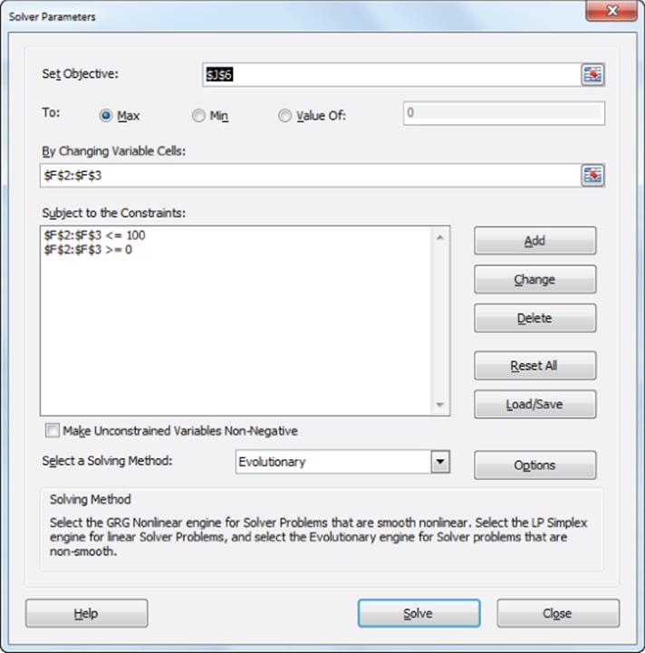
You need to constrain the fixed and variable costs between $0 and $100. The profit is maximized by charging a fixed fee of $60.27 and a cost of $2.21 per unit. Again a maximum profit of $64 is made, and the customer purchases 16 units.
All three of the fairly simple nonlinear pricing strategies result in doubling the linear price profit to $64. There is no nonlinear pricing plan that can make more than $64 off the customer. You can easily show the exact value of the sixteenth unit is $2.25, and the exact value of the seventeenth unit is $1.75, which is less than the unit cost of $2.00. Because the customer values unit 16 more than the cost, you should be able to get her to buy 16 units. Because the area under the demand curve (see Exercise 5) from 0 to 16 is 96, the most you can make the consumer pay for 16 units is $96. Therefore your maximum profit is $96 – ($2)(16) = $64, which is just what you obtained using all three nonlinear pricing strategies. The problem with the linear pricing strategy is that it does not extract the surplus value in excess of the $2 cost that the customer places on earlier units. The nonlinear pricing strategies manage to extract all available consumer surpluses.
For a monopolist (like a power company) it may be realistic to assume that an organization can extract all consumer surplus. In the presence of competition, it may be unrealistic to assume that an organization can extract all consumer surplus. To illustrate how the models of this chapter can be modified in the presence of competition, suppose you are planning to enter a business where there is already a single company selling a product. Assume that this company is currently extracting 80 percent of the consumer surplus and leaving 20 percent of the consumer surplus with the consumer. By adding a constraint to your models that leaves, say 25 percent of the consumer surplus in the hands of the customer, you can derive a reasonable nonlinear pricing strategy that undercuts the competition. For an illustration of this idea see Exercise 8.
Summary
In this chapter you learned the following:
· Nonlinear pricing strategies involve not charging the same price for each unit sold.
· If you assume customers purchase the available option with the largest (if non-negative) surplus, then you can use the Evolutionary Solver to find profit maximizing nonlinear pricing strategies such as quantity discounts and two-part tariffs.
· For a linear demand curve, nonlinear pricing earns twice as much profit as linear pricing.
Exercises
1. You own a small country club. You have three types of customers who value each round of golf they play during a month as shown in the following table:
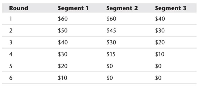
It costs you $5 in variable costs to provide a customer with a round of golf. Find a profit maximizing a two-part tariff. Each market segment is of equal size.
The demand curve for a product is q = 4000 − 40p. It costs $5 to produce each unit.
a. If you charge a single price for each unit, how can you maximize profit?
b. If you use a two-part tariff, how can you maximize the profit?
3. Using the data in Exercise 1, determine the profit maximizing the quantity discount scheme in which all units up to a point sell for a high price, and all remaining units sell for a low price.
4. The file Finalmusicdata.xls (available on the companion website) contains data showing the most 1,000 people were willing to pay for 10 songs. For example, as shown in Figure 6.7, Person 1 is willing to pay up to 38 cents for Song 1.
Figure 6-7: Data for Problem 4
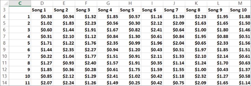
a. If you charge a single price for each song, what price can maximize your revenue?
b. If you use a two-part tariff pricing scheme (for example $3 to download any songs + 40 cents per song), how can you maximize revenue?
c. How much more money do you make with the two-part tariff?
NOTE
For the second part, you must realize that a person will buy either nothing, their top-valued song, their top 2 songs, their top 3 songs,…their top 9 songs or top 10 songs.
5. Show that for the demand curve q = 40 – 2p the consumer places a value of exactly $256 on the first 16 units.
6. (Requires calculus) Suppose the demand for a computer by a leading corporate client (for p≥100) is given by 200000 / p2. Assume the cost of producing a computer is $100.
a. If the same price is charged for each computer, what price maximizes profit?
b. If you charge HP for the first CUT computers and LP for remaining computers purchased, how can you maximize profit?
7. Suppose Verizon has only three cell phone customers. The demand curve for each customer's monthly demand (in hours) is shown here:
|
Customer |
Demand curve |
|
1 |
Q = 60 – 20p |
|
2 |
Q = 70 – 30p |
|
3 |
Q = 50 – 8p |
Here p = price in dollars charged for each hour of cell phone usage. It costs Verizon 25 cents to provide each hour of cell phone usage.
a. If Verizon charges the same price for each hour of cell phone usage, what price should they charge?
b. Find the profit maximizing a two-part tariff for Verizon. How much does the best two-part tariff increase the profit over the profit maximizing the single price?
8. For the power company example construct a standard quantity discount pricing strategy that leaves the customer with 25 percent of the consumer surplus.
All materials on the site are licensed Creative Commons Attribution-Sharealike 3.0 Unported CC BY-SA 3.0 & GNU Free Documentation License (GFDL)
If you are the copyright holder of any material contained on our site and intend to remove it, please contact our site administrator for approval.
© 2016-2026 All site design rights belong to S.Y.A.