Marketing Analytics: Data-Driven Techniques with Microsoft Excel (2014)

Part II. Pricing

Chapter 8. Revenue Management

Often you purchase an item that seems identical and the price changes. Here are some examples:

· When I fly from Indianapolis to Los Angeles to visit my daughter, the price I have paid for a roundtrip ticket has varied between $200 and $900.

· When I stay in LA at the downtown Marriott, I usually pay $300 per night for a weekday and under $200 a night for a weekend.

· When I rent a car from Avis on a weekend I pay much less than the weekday rate.

· The day after Easter I can buy Easter candy much cheaper than the day before!

· My local steakhouse offers a second entrée for half price on Monday–Wednesday.

· It is much cheaper to rent a house in Key West, Florida in the summer than during the winter.

· The Indiana Pacers charge much more for a ticket when they play the Heat.

· Movies at my local theater cost $5 before 7 p.m. and $10 after 7 p.m.

All these examples illustrate the use of revenue management. Revenue management (often referred to as yield management) is used to describe pricing policies used by organizations that sell goods whose value is time-sensitive and usually perishable. For example, after a plane takes off, a seat on the plane has no value. After Easter, Easter candy has reduced value. On April 2, an April 1 motel room has no value.

Revenue management has increased the bottom line for many companies. For example:

· American Airlines credits revenue management with an annual revenue increase of $500 million.

· In 2003, Marriott reported revenue management increased profit by $6.7 million.

· Revenue management is credited with saving National Rental Car from bankruptcy.

This chapter explains the basic ideas behind revenue management. The reader who wants to become an expert in revenue management should read Kalyan Talluri and Garrett Ryzin's treatise (The Theory and Practice of Revenue Management (Springer-Verlag, 2004).

The main revenue management concepts discussed in this chapter are the following:

· Making people pay an amount close to their actual valuation for a product.For example, business travelers are usually willing to pay more for a plane ticket, so revenue management should somehow charge most business travelers a higher price than leisure travelers for a plane ticket.

· Understanding how to manage the uncertainty about usage of the perishable good.For example, given that some passengers do not show up for a flight, an airline needs to sell more tickets than seats on the plane, or else the plane leaves with some empty seats.

· Matching a variable demand to a fixed supply.For example, power companies will often charge more for power during a hot summer day in an attempt to shift some of the high power demand during the afternoon to the cooler evening or morning hours.

Estimating Demand for the Bates Motel and Segmenting Customers

In many industries customers can be segmented based on their differing willingness to pay for a product. For example, business travelers (who do not stay in their destination on Saturday nights) are usually willing to pay more for a plane ticket than non-business travelers (who usually stay in their destination on Saturday.) Similarly business travelers (who often reserve a room near the reservation date) often are willing to pay more for a hotel room than a non-business traveler (who usually reserves the room further in advance.) This section uses an example from the hotel industry to show how a business can increase revenue and profit by utilizing the differing valuations of different market segments.

Estimating the Demand Curve

Suppose the 300-room Bates Motel wants to maximize its revenue for June 15, 2016. They asked 2 percent (10 people) of the potential market (business has dropped at the Bates Motel since an incident in 1960) their valuation for a stay at the Motel on June 15, 2016, and found the results shown inFigure 8.1. This work is in the demand curve worksheet of the file Batesmotel.xlsx.

Figure 8-1: Estimating Bates Motel demand curve

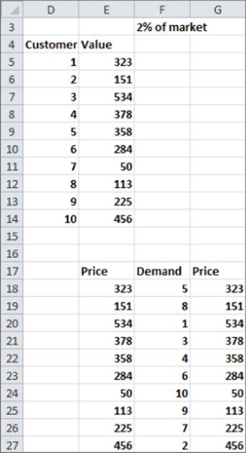
You can estimate a demand curve for June 15, 2016, after you have 10 points on the demand curve. For example, 5 of the 10 people have valuations of at least $323, so if you charge $323 for a room, 2 percent of your demand equals 5. To compute 10 points on the demand curve, simply list the 10 given valuations in E18:E27. Then copy the formula =COUNTIF($E$5:$E$14,">="&E18) from F18 to F19:F27. In cell F18, for example, this formula counts how many people have valuations at least as large as $323.

You can now use the Excel Trend Curve to find the straight-line demand curve that best fits the data. To do so, follow these steps:

1. Enter the prices again in the cell range G18:G27 so that you can fit a demand curve with quantity on the x-axis and price on the y-axis.

2. Select the range F18:G27 and then on the ribbon navigate to Insert &cmdarr; Charts &cmdarr; Scatter. Choose the first option (just dots) to obtain a plot of demand against price.

3. Right-click the series; select Add Trendline… and choose the Linear option. Then check Display Equation on chart. This yields the chart shown in Figure 8.2, which shows the best-fitting linear demand curve p = 564.87-50.49 * q.

Figure 8-2: Chart of Bates Motel demand curve

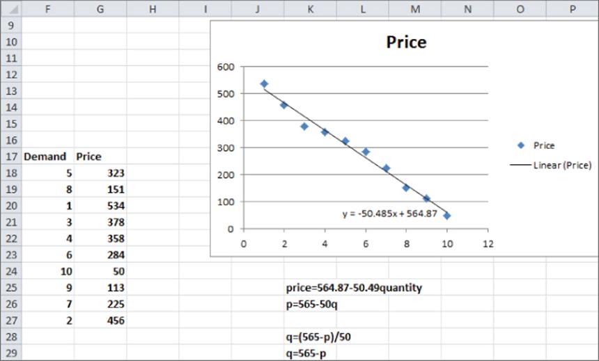
4. Round this off to simplify calculations; you can assume the demand curve is p = 565 − 50q.

5. Solve for q in terms of p; you find: .

6. Because this is 2 percent of your demand, multiply the previous demand estimate by 50. This cancels out the 50 in the denominator and you find your entire demand is given by q = 565 − p.

Optimal Single Price

To show how revenue management increases profits, you need to determine profits when revenue management is not applied; that is, when each customer is charged the same price.

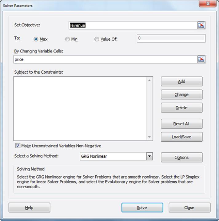
To simplify your approach, temporarily ignore the 300-room capacity limitation. Under this assumption, if the Bates Motel wants to maximize profit, it should simply choose a price to maximize: profit = price * (565-price). The approach described in Chapter 4, “Estimating Demand Curves and Using Solver to Optimize Price” is now used to determine a single profit maximizing price. The work is in the single price worksheet of the Batesmotel.xslx file as shown in Figures 8.3 and the Solver window in Figure 8.4. Maximum revenue of $79,806.25 is obtained by charging a price of $282.50.

Figure 8-3: Computing the best single price

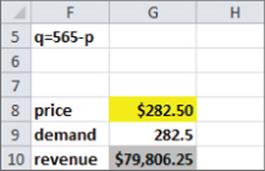
Figure 8-4: Solver window to find best single price

Using Two Prices to Segment Customers

To maximize revenue the Bates Motel would love to charge each customer an individual valuation. However, this is illegal; each customer must be charged the same price. Yield management, however, provides a legal way to price discriminate and increase profits.

If there is a variable highly correlated with a customer's willingness to pay, then Bates can approximate the individual pricing strategy. Suppose that low-valuation customers are willing to purchase early, and high-value customers usually purchase near the date of the reservation. Bates can approximate the individual pricing strategy by charging a price low for advance purchases and a price high for last minute purchases. Assuming that all customers with high valuations arrive at the last minute this would result in a demand 565 − high for last-minute sales and a demand (565 − low) − (565 − high) for advance sales. The Solver model to determine the revenue maximizing high and low prices is in the Segmentation worksheet (see Figure 8.5.) You proceed as follows:

1. In cell F12 compute the demand for last-minute reservations with the formula =565-high.

2. In cell F13 compute the advance demand with the formula =(565-low)-(565-high).

3. In cell F14 compute the revenue from last-minute reservations with the formula =high*highdemand.

4. In cell F15 compute the revenue from advance reservations with the formula =lowdemand*low.

5. In cell F16 compute the total revenue with the formula =SUM(F14:F15).

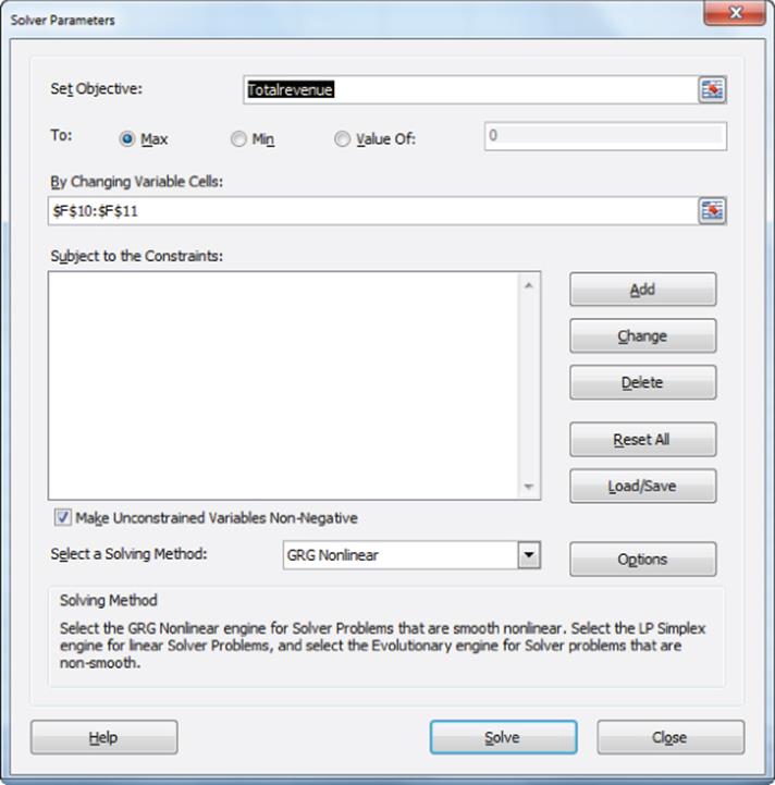
6. As shown in the Solver window (refer to Figure 8.6), you choose non-negative high and low prices to maximize total revenue.

Figure 8-5: Model for computing prices with segmentation

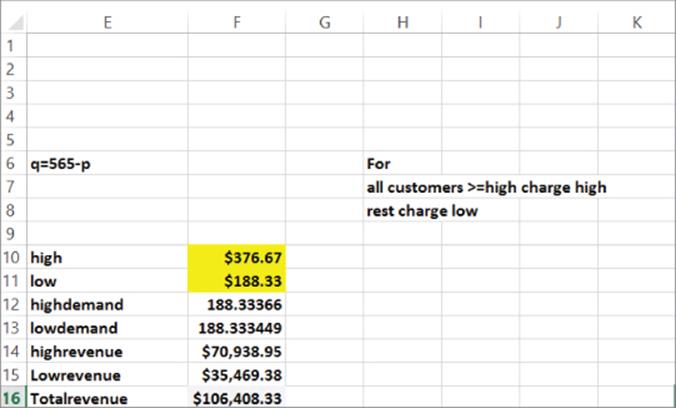
Figure 8-6: Solver window with segmentation

You'll find that a high price of $376.67 should be charged for last-minute reservations and a low price of $188.33 for advance reservations. Bates' revenue has now increased by 33 percent to $106,408.33. Of course, this revenue increase would be realized only if there were a perfect correlation between willingness to pay and a customer wanting to buy in advance at the last minute. If this correlation existed, it provides a legal way for Bates to charge higher prices to high-valuation customers. In this situation, Bates can add a qualifying restriction (say, reserve rooms at least 2 weeks in advance) or a fence, that separates high-valuation and low-valuation customers. Airlines often use similar tactics by using the qualifying restriction of “staying over a Saturday night” as an imperfect fence to separate leisure and business travelers.

This solution, however, resulted in more people showing up than the hotel has rooms. You can resolve this issue by adding constraints on received reservations.

Segmentation with Capacity Constraints

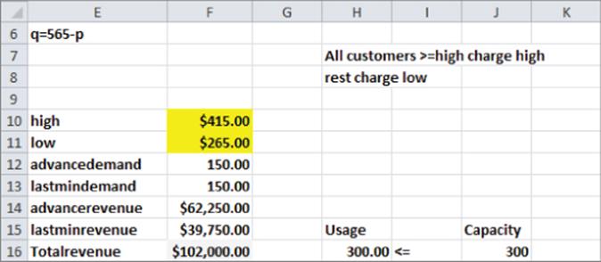
In Figure 8.7, you can see how to ensure that the number of rooms reserved will not exceed capacity. After all you don't want Norman to stay in his mother's room. To avoid this problem, copy the Segmentation worksheet to a new worksheet named Segmentation with capacity. Then compute total rooms reserved in cell H16 and add a constraint that H16<=J16. As shown in Figure 8.7, $415 should be charged for last-minute reservations and $265 for advance reservations. One hundred and fifty reservations of each type will be purchased and the revenue drops by approximately 4 percent to $102,000. Note that the new prices result in the number of reservations equaling capacity.

Figure 8-7: Optimal prices with capacity restriction

Handling Uncertainty

The analysis of the Bates Motel in the previous section implicitly assumed that when prices were set Bates knew exactly how many people would reserve in advance and at the last minute. Of course, this is not the case. In this section you learn how Bates should deal with this uncertainty. When developing revenue management systems, airlines also deal with uncertainty, such as the number of people that will fail to show up for a flight.

Determining a Booking Limit

To illustrate the role of uncertainty in revenue management, assume all advance reservations arrive before all last-minute reservations. Bates charges $105 for an advance reservation and $159 for a last-minute reservation. Also assume that sufficient customers want to reserve in advance to fill all the rooms. Because Bates does not know how many last-minute reservations will occur, it “protects” a certain number of rooms for last-minute reservations. A protection limit is the number of rooms not sold to advance reservations because late arrivals are willing to pay more for a room. Alternatively, a booking limit is the maximum number of rooms reserved for advance purchases. For example, a booking limit of 200 means Bates will allow at most 200 rooms to be reserved at the $105 price. Of course a booking limit of 200 rooms is equivalent to a protection limit of 300 – 200 = 100 rooms.

Assume the number of last-minute reservations that Bates receives is unknown and follows a normal random variable with a mean of 100 and a standard deviation of 20. This implies there is a 68 percent chance that between 80 and 120 last-minute reservations will be received, and a 95 percent chance that between 60 and 140 last-minute reservations will be received.

Now you can determine the protection level Q that maximizes Bates' expected profit using the powerful concept of marginal analysis. In marginal analysis you try and determine an optimal value of a decision variable by comparing the benefits of a unit change in the variable to the cost incurred from a unit change in a variable. To apply marginal analysis to the determination of the optimal protection level you check if for a given value of Q, Bates can benefit by reducing the protection level from Q + 1 to Q. To do so perform these steps:

1. Define F(Q) the probability number of last-minute reservations as less than or equal to Q, or F(Q)=n(last minute reservations)≥Q.

2. Because you assumed all rooms could be filled at the discounted price, reducing the protection level by 1 would surely gain Bates $105.

3. With probability 1 – F(Q) Bates would sell the Q +1 protected room at a $159 price, so on average Bates would lose (1-F(Q))*159+F(Q)*0 =(1-F(Q))*159 if it reduces the protection level by 1. Therefore Bates should reduce the protection level from Q+1 to Q if and only if 105>=(1-F(Q))*159 or F(Q)>=54/159=.339.

4. You can find the 33.9 percentile of last-minute reservations using the Excel NORMINV function. NORMINV(probability, mean, standard_dev) gives the value Q for a normal random variable with a given mean and standard deviation such that F(Q)=p. Enter =NORMINV(0.339,100,20) into Excel. This yields 91.70. Therefore F(91)<.339 and F(92)>.339, so Bates Motel should protect 92 rooms.

Overbooking Models

Airlines usually have several fare classes, so they must determine more than one booking limit. As the time of the flight approaches, airlines update the booking limits based on the number of reservations received. This updating requires lots of past data on similar flights. In most cases, revenue management requires a large investment in information technology and data analysis, so the decision to institute a revenue management program should not be taken lightly.

Airlines always deal with the fact that passengers who have a ticket may not show up. If airlines do not “overbook” the flight by selling more tickets than seats, most flights leave with empty seats that could have been filled. Of course, if they sell too many tickets, they must give “bumped” passengers compensation, so airlines must trade off the risk of empty seats against the risk of overbooking. Marginal analysis can also be used to analyze this trade-off problem.

To illustrate the idea, suppose the price for a New York to Indianapolis flight on Fly by Night (FBN) airlines is $200. The plane seats 100 people. To protect against no-shows, FBN tries to sell more than 100 tickets. Federal Law requires that any ticketed customer who cannot board the plane is entitled to $100 compensation. Past data indicates the number of no-shows for this flight follows a normal random variable with mean 20 and standard deviation 5. To maximize expected revenue less compensation costs for the flight, how many tickets should FBN try to sell for each flight? Assuming that unused tickets are refundable, follow these steps:

1. Let Q equal number of tickets FBN will try to sell and NS equal number of no shows. You can model NS as a continuous random variable, so NS can assume a fractional value. Therefore assume, for example, that if Q – NS is between 99.5 and 100.5, then 100 passengers will show up.

2. For a given value of Q, consider whether you should reduce Q from Q + 1 to Q. If Q – NS >= 99.5, then you save $100 by reducing ticket limit from Q + 1 to Q. This is because one less person will be overbooked. On the other hand, if Q – NS<99.5, then reducing the ticket limit from Q + 1 to Q results in one less ticket sale, which reduces revenue by $200. If F(x) = Probability number of no-shows is less than or equal to x, then

· With Probability F(Q – 99.5) reducing the ticket limit from Q + 1 to Q saves $100.

· With probability 1 – F(Q – .99.5) reducing the ticket limit from Q +1 to Q costs $200.

Therefore reducing the ticket limit from Q + 1 to Q benefits you if:

Or

3. Now NORMINV(0.667,20,5)=22.15. This implied that if and only if Q – 99.5 >= 22.15 or Q >= 121.65 you should reduce Q from Q + 1 to Q. Therefore you should reduce tickets sold from 123 to 122 and stop there. In short, to maximize expected revenue less compensation costs, FBN should cut ticket sales off at 122 tickets.

The problem faced by the airlines is much more complicated than this simple overbooking model. At every instant the airline must update their view of how many tickets will be sold for the flight and use this information to determine optimal decisions on variables such as booking limits.

Markdown Pricing

Many retailers practice revenue management by reducing a product's price based on season or timing. For example, bathing suits are discounted at the end of the summer. Also Easter candy and Christmas cards are discounted after the holiday. The now defunct Filene's Basement of Boston for years used the following markdown policy:

· Twelve days after putting an item on sale, the price was reduced by 25%.

· Six selling days later, the price is cut by 50%.

· After an additional 6 selling days, the items were offered at 75% off the original price.

· After 6 more selling days, the item was given to charity.

The idea behind markdown pricing is that as time goes on, the value of an item to customers often falls. This logic especially applies to seasonal and perishable goods. For example, a bathing suit purchased in April in Indiana has much more value than a bathing suit purchased in September because you can wear the April-purchased suit for many more upcoming summer days. Likewise, to keep perishable items from going bad before they are sold supermarkets markdown prices when a perishable item gets near its expiration date. Because customers only buy products if perceived value exceeds cost, a reduction in perceived value necessitates a reduction in price if you still want to maintain a reasonable sales level. The following example further illustrates mark-down pricing.

Consider a store that sells a product (such as swimsuits) over a three-month period. The product is in demand most when it first hits the stores. In the workbook Markdownpricing.xlsx you will determine how pricing strategy maximizes profit. Figure 8.8 shows the markdown pricing spreadsheet model.

Figure 8-8: Markdown pricing model

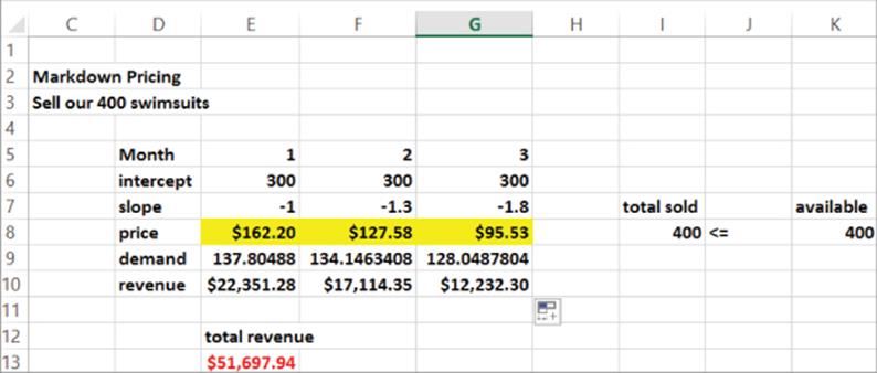
Suppose you have 400 swimsuits to sell and the methods of Chapter 4 have been used to estimate the following demand curves:

· Month 1 Demand = 300 – price

· Month 2 Demand = 300 – 1.3price

· Month 3 Demand = 300 – 1.8price

To determine the sequence of prices that maximizes your revenue, proceed as follows (see the order 400 worksheet):

1. Solver requires you to start with numbers in the changing cells, so in E8:G8 enter trial values for each week's price.

2. Copy the formula =E6+E7*E8 from E9 to E9:G9 to generate the actual demand each month.

3. Copy the formula =E8*E9 from E10 to F10:G10 to compute each month's revenue.

4. The total revenue is computed in cell E13 with the formula =SUM(E10:G10).

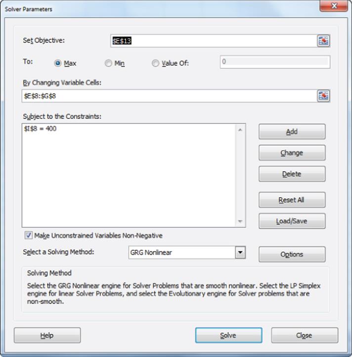
You can maximize revenue (E13) by changing prices (E8:G8) and constrain units sold (I8) to equal 400. The Solver window is shown in Figure 8.9.

Figure 8-9: Solver window for markdown pricing

A maximum revenue of $51,697.94 is obtained by charging $162.20 during Month 1, $127.58 during Month 2, and $95.53 during Month 3. Of course, the prices are set to ensure that all 400 swimsuits are sold.

Your model would be more realistic if the store realizes that it should also try to optimize the number of swimsuits it buys at the beginning of the season. Assume the store must pay $100 per purchased swimsuit. In the how many worksheet (see Figure 8.10) you can use Solver to determine prices that maximize profit.

Figure 8-10: Markdown pricing and purchase decision

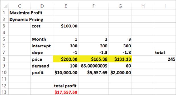
In E10:G10 you can revise the profit formulas to include the purchase cost by copying the formula =(E8 –cost)*E9 from E10 to F10:G10. After deleting the constraint I8 = 400, the Solver window is identical to Figure 8.9. Profit is maximized at a value of $17,557.69 by buying 245 swimsuits and charging $200 in Month 1, $165.38 in Month 2, and $133.33 in Month 3.

Summary

In this chapter you learned the following:

· Revenue management enables organizations including airlines, hotels, rental car agencies, restaurants, and sports teams to increase profits by reducing the unused amount of perishable inventory (seats, hotel rooms, and so on) Revenue management also enables organizations to better match the price charged to customers with what they are willing to pay.

· Revenue management has a much greater chance of succeeding if “fences” (such as staying over Saturday night for airlines) exist to separate high-valuation customers from low-valuation customers.

· To handle the fact that organizations do not know how many high-value customers will demand a product, organizations often set booking limits to constrain low-price sales so that more capacity is reserved for late arriving high-valuation customers.

· To adjust for the possibility of no shows, organizations need to sell more capacity than is available.

· Marginal analysis is helpful to solve booking limits and overbooking problems.

· Often the valuation customers have for products drops over time. This requires that retailers lower or mark down their prices over time.

Exercises

1. Redo the analysis in the first section, “Estimating Demand for the Bates Motel and Segmenting Customers,” assuming demand follows a constant elasticity demand curve. Use the Power Curve option on the Excel Trendline to fit the demand curve.

2. How can TV networks use revenue management?

3. How can Broadway plays use revenue management?

4. A flight from New York to Atlanta has 146 seats. Advance tickets purchased cost $74. Last-minute tickets cost $114. Demand for full-fare tickets is normally distributed with a mean of 92 and standard deviation of 30. What booking limit maximizes expected revenues? Assume there are no no-shows and always enough advanced purchasers to fill the flight.

5. Suppose a Marriot offers a $159 discount rate for a midweek stay. Its regular rate is $225. The hotel has 118 rooms. Suppose it is April 1 and the Marriott wants to maximize profit from May 29 bookings. The Marriott knows it can fill all rooms at the discounted price, but to maximize profit it must reserve or protect some rooms at the high price. Because business travelers book late, the hotel decides to protect or reserve rooms for late-booking business customers. The question is how many rooms to protect. The number of business travelers who will reserve a room is unknown, and you can assume it is normal with the mean = 27.3 and a standard deviation of 6. Determine the Protection Limit that maximizes the expected profit. Again assume that there are always enough leisure travelers to pay the discount rate for the unsold rooms.

6. The Atlanta to Dallas FBN flight has 210 seats and the fare is $105. Any overbooked passenger costs $300. The number of no-shows is normal with a mean of 20 and standard deviation of 5. All tickets are nonrefundable. How many reservations should FBN accept on this flight?

7. The pre-Christmas demand for Christmas cards at a local Hallmark stores is given by q = 2000 – 300p. The demand for Christmas cards after Christmas is given by q = 1000 – 400p. If the store pays $1 per card, how can they maximize profits from Christmas cards? Assume they want all inventory sold.