Excel 2016 All-in-One For Dummies (2016)

Book II

Worksheet Design

Check out the article “Selecting Cells with the Keyboard in Excel 2016” online at www.dummies.com/extras/excel2016aio.

Contents at a Glance

1. Chapter 1: Building Worksheets

1. Designer Spreadsheets

2. It Takes All Kinds (Of Cell Entries)

3. Data Entry 101

4. Saving the Data

5. Document Recovery to the Rescue

2. Chapter 2: Formatting Worksheets

1. Making Cell Selections

2. Adjusting Columns and Rows

3. Formatting Tables from the Ribbon

4. Formatting Tables with the Quick Analysis Tool

5. Formatting Cells from the Ribbon

6. Formatting Cell Ranges with the Mini-Toolbar

7. Using the Format Cells Dialog Box

8. Hiring Out the Format Painter

9. Using Cell Styles

10. Conditional Formatting

3. Chapter 3: Editing and Proofing Worksheets

1. Opening a Workbook

2. Cell Editing 101

3. A Spreadsheet with a View

4. Copying and Moving Stuff Around

5. Find and Replace This Disgrace!

6. Spell Checking Heaven

7. Looking Up and Translating Stuff

8. Marking Invalid Data

9. Eliminating Errors with Text to Speech

4. Chapter 4: Managing Worksheets

1. Reorganizing the Worksheet

2. Reorganizing the Workbook

3. Working with Multiple Workbooks

4. Consolidating Worksheets

5. Chapter 5: Printing Worksheets

1. Printing from the Excel 2016 Backstage View

2. Quick Printing the Worksheet

3. Working with the Page Setup Options

4. Headers and Footers

5. Solving Page Break Problems

6. Printing the Formulas in a Report

Chapter 1

Building Worksheets

In This Chapter

Creating a spreadsheet from a template

Designing a spreadsheet from scratch

Understanding the different types of cell entries

Knowing the different ways of entering data in the worksheet

Using Data Validation to restrict the data entries in cells

Saving worksheets

Before you can begin building a new spreadsheet in Excel, you must have the design in mind. As it turns out, the design aspect of the creative process is often the easiest part because you can borrow the design from other workbooks that you’ve already created or from special workbook files, called templates, which provide you with the new spreadsheet’s form along with some of the standard, or boilerplate, data entries.

After you’ve settled upon the design of your new spreadsheet, you’re ready to begin entering its data. In doing the data entry in a new worksheet, you have several choices regarding the method to use. For this reason, this chapter not only covers all the methods for entering data — from the most basic to the most sophisticated — but also includes hints on when each is the most appropriate. Note, however, that this chapter doesn’t include information on building formulas, which comprises a major part of the data entry task in creating a new spreadsheet. Because this task is so specialized and so extensive, you find the information on formula building covered in Book III, Chapter 1.

Designer Spreadsheets

Anytime you launch Excel (without also opening an existing workbook file), the Excel screen in the Backstage view presents you with a choice between

· Opening a new workbook (with the generic filename, Book1), consisting of a single totally blank worksheet (with the generic worksheet name, Sheet1) by selecting the Blank Workbook template

· Opening a new workbook based on the design in one of the other templates displayed in the Start screen or available for download by conducting an online search

If you select the Blank Workbook template, you can start laying out and building your new spreadsheet in the blank worksheet. If you select one of the other designed templates, you can start by customizing the workbook file’s design as well as entering the data for your new spreadsheet.

Take it from a template

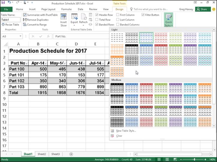
Spreadsheet templates are the way to go if you can find one that uses the design of the spreadsheet that you want to build. There are many templates to choose from when you initially launch Excel. (See Figure 1-1.) The templates displayed on the Excel screen in the Backstage view run the gamut from budgets and schedules to profit and loss statements, sales reports, and calendars.

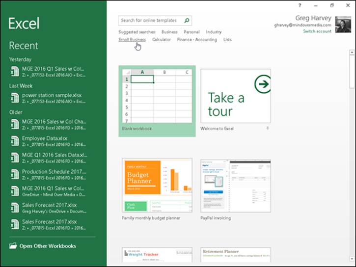
Figure 1-1: Selecting a template from which to generate a new workbook in the Excel Start screen.

If none of the templates displayed on the Excel screen fit the bill, you can then search for templates. This screen contains links to common suggested searches: Business, Personal, Industry, Small Business, Calculator, Finance-Accounting, and Lists.

When you click one of these links, a New screen appears in the Backstage view showing your choices in that particular category. Figure 1-2 shows you the New screen that appears when you click the Small Business link in the Suggested Searches area of the Start screen. As you can see in this figure, the first choice in this category is an Invoice template that automatically calculates totals that you can download and open in Excel 2016.

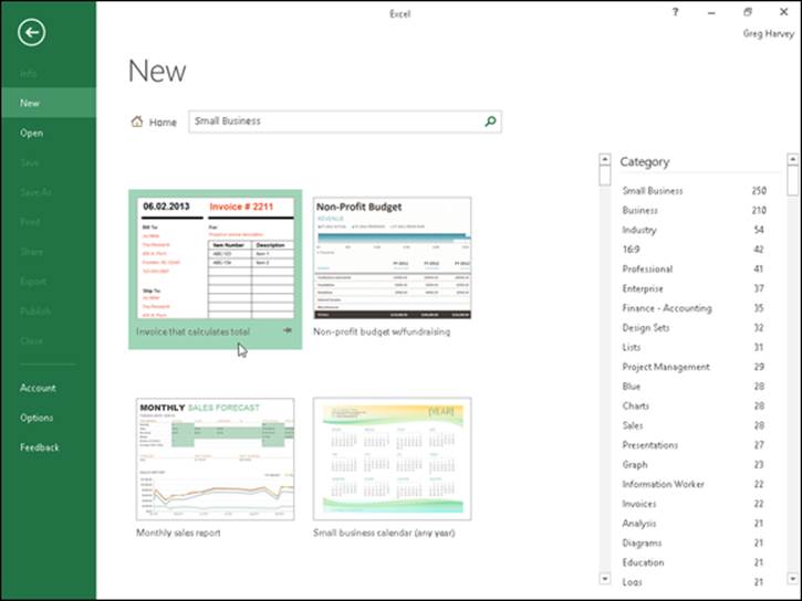
Figure 1-2: Searching for an Invoice template using the Small Business link in Suggested Searches on the Start screen.

If the type of template you’re looking for doesn’t fit any of the categories listed in the Suggested Searches area of the Excel screen, you conduct your own template search. Simply select the Search for Online Templates text box, type in keywords describing the type of template (such as expense report), and then select the Start Searching button (the one with the magnifying glass icon).

Keep in mind that instead of using ready-made templates, you can create your own templates from your favorite Excel workbooks. After you save a copy of a workbook as a template file, Excel automatically generates a copy of the workbook whenever you open the template file. This way, you can safely customize the contents of the new workbook without any danger of inadvertently modifying the original template.

Downloading the template to use

When you locate a template whose design can be adapted to your spreadsheet needs, you can download it. Simply click its thumbnail in the Excel or New screen. Excel then opens a dialog box similar to the one shown in Figure 1-3, containing a more extensive description of the template and its download file size. To download the template and create a new Excel workbook from it, you simply select the Create button.

Figure 1-3: Downloading a Weekly Expense Report template from which to generate a new workbook.

Figure 1-4 shows the Weekly Expense Report1 workbook in the Excel worksheet area created from the Expense Report template after you click the Create button. As you can see on the Excel window title bar in this figure, when Excel generated this first workbook from the original template file, the program also gave it the temporary filename, Weekly Expense Report1. If you were to then create a second copy of this report by once again opening the Expense Report template, the program would name that copy Weekly Expense Report2. This way, you don’t have to worry about one copy overwriting another, and you never risk mistakenly saving changes to the original template file itself (which actually uses a completely different filename extension — .xltx for an Excel template as opposed to .xlsx for an Excel worksheet).

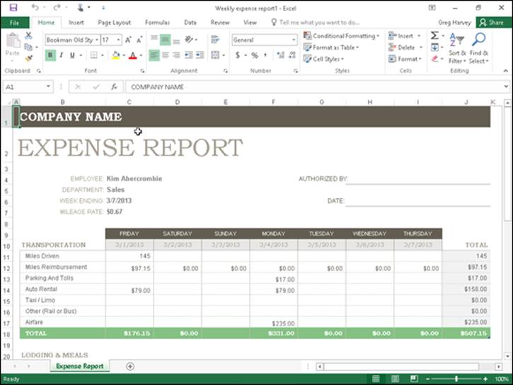
Figure 1-4: The new Weekly Expense Report1 workbook in the Excel worksheet area generated from the template by the same name.

To customize a spreadsheet generated from one of the installed templates, you replace the placeholder entries in the new sales worksheet with your own data. You might begin by replacing the COMPANY NAME placeholder in cell A1 with the actual name of your company, after which you could replace the employee name Kim Abercrombie in cell C4, with your own name (unless, of course, your name just happens to be Kim Abercrombie). Then, you would start replacing the placeholder dates with your own dates and the mileage figures with actual miles driven. For strategies on entering your labels and values into the cells of a worksheet, see “It Takes All Kinds (Of Cell Entries)” later in this chapter.

Note that when filling in or replacing the data a spreadsheet generated from one of these ready-made templates, you have access to all the cells in the worksheet: those that contain standard headings as well as those that require personalized data entry.

After you finish filling in the personalized data, save the workbook just as you would a workbook that you had created from scratch. (See the “Saving the Data” section at the end of this chapter for details on saving workbook files.)

Saving changes to your customized templates

You can save the customization you do to the templates you download to make the workbooks you create from them easier to use and quicker to fill out. For example, you can make your own custom Weekly Expense Report template from one generated by the downloaded template by filling in your company name and address in the top section and your billing terms and a thank-you message in the bottom sections.

To save your changes to a downloaded template as a new template file, follow these steps:

1. Click the Save button on the Quick Access toolbar (the one with the disk icon), or choose File  ⇒  Save from the File menu button, or press Ctrl+S.

The Save As screen opens where you select the location where the customized template file is to be saved.

2. Select the drive and folder where you store all your personal template files in the Save As screen.

This personal templates folder can be local on your OneDrive. However, you need to mark its location (because later on you need to enter its pathname in the Excel Options dialog box), and you need to designate it as the place in which to save all personal templates you create in the future.

As soon as you select the folder and drive in which to save your template, Excel opens the Save As dialog box, where you need to change the file type from a regular Microsoft Excel Workbook (*.xlsx) to ExcelTemplate (*.xltx) in the Save as Type drop-down list box.

3. Click the Save as Type drop-down button and then select Excel Template from the drop-down list.

If you need your new template file to be compatible with earlier versions of Excel (versions 97 through 2003), select Excel 97-2003 Template (*.xlt) rather than Excel Template (*.xltx) from the Save as Type drop-down list. When you do this, Excel saves the new template file in the older binary file format (rather than the newer XML file format) with the old .xlt filename extension instead of the newer .xltx filename extension. If your template contains macros that you want the user to be able to run when creating the worksheet, select Excel Macro-Enabled Template (*.xltm).

4. Click in the File Name text box and then modify the default filename as needed before you select the Save button to close the Save As dialog box and save your customized template in the Templates folder.

After the Save As dialog box closes, you still need to close the customized template file in the Excel work area.

5. Choose File  ⇒  Close, or press Alt+FC, or press Ctrl+W to close the customized template file.

After saving an initial customized template file in your personal template folder, you need to tell Excel about this folder and where it is by following these steps:

1. Choose File  ⇒  Options  ⇒  Save (Alt+FTS).

Excel opens the Excel Options dialog box and selects the Save tab.

2. Click the Default Personal Templates Location text box and enter the complete filename path for the folder where you saved your initial personal template file.

For example, if I created a Templates folder within the Documents folder on my personal OneDrive where I save all my personal Excel template files, I would enter the following pathname in the Default Personal Templates Location text box:

C:\Users\Greg\OneDrive\Documents\Templates

3. Click OK to close the Excel Options dialog box.

After designating the location of your personal templates folder as described in the preceding steps, the next time you open the Excel or New screen in the Excel Backstage, two links, Featured and Personal, now appear under the Suggested Searches headings (see Figure 1-1). To generate a new workbook from one of your custom spreadsheet templates, you click the Personal link to display thumbnails for all the templates saved in the designated personal templates folder. To open a new Excel workbook from one of its custom templates, you simply click its thumbnail image.

Creating your own spreadsheet templates

You certainly don’t have to rely on spreadsheet templates created by other people. Indeed, many times you simply can’t do this because, even though other people may generate the type of spreadsheet that you need, their design doesn’t incorporate and represent the data in the manner that you prefer or that your company or clients require.

When you can’t find a ready-made template that fits the bill or that you can easily customize to suit your needs, create your own templates from sample workbooks that you’ve created or that your company has on hand. The easiest way to create your own template is to first create an actual workbook prototype, complete with all the text, data, formulas, graphics, and macros that it requires to function.

When readying the prototype workbook, make sure that you remove all headings, miscellaneous text, and numbers that are specific to the prototype and not generic enough to appear in the spreadsheet template. You may also want to protect all generic data, including the formulas that calculate the values that you or your users input into the worksheets generated from the template and headings that never require editing. (See Book IV, Chapter 1 for information on how to protect certain parts of a worksheet from changes.)

After making sure that both the layout and content of the boilerplate data are hunky-dory, save the workbook in the template file format (.xltx) in your personal templates folder so that you can then generate new workbooks from it. (For details on how to do this, refer to the steps in the previous section, “Saving changes to your customized templates.”)

As you may have noticed when looking through the sample templates included in Excel (refer to Figure 1-4, for example) or browsing through the templates that you can download from the Microsoft Office.com website found at http://office.microsoft.com, many spreadsheet templates abandon the familiar worksheet grid of cells, preferring a look very close to that of a paper form instead. When converting a sample workbook into a template, you can also remove the grid, use cell borders to underscore or outline key groups of cells, and color different cell groups to make them stand out. (For information on how to do this kind of stuff, refer to Book II, Chapter 2.)

Keep in mind that you can add online comments to parts of the template that instruct co-workers on how to properly fill in and save the data. These comments are helpful if your co-workers are unfamiliar with the template and may be less skilled in using Excel. (See Book IV,Chapter 3 for details about adding comments to worksheets.)

Designing a workbook from scratch

Not all worksheets come from templates. Many times, you need to create rather unique spreadsheets that aren’t intended to function as standard models from which certain types of workbooks are generated. In fact, most of the spreadsheets that you create in Excel may be of this kind, especially if your business doesn’t rely on the use of highly standardized financial statements and forms.

Planning your workbook

When creating a new workbook from scratch, you need to start by considering the layout and design of the data. When doing this mental planning, you may want to ask yourself some of the following questions:

· Does the layout of the spreadsheet require the use of data tables (with both column and row headings) or lists (with column headings only)?

· Do these data tables and lists need to be laid out on a single worksheet or can they be placed in the same relative position on multiple worksheets of the workbook (like pages of a book)?

· Do the data tables in the spreadsheet use the same type of formulas?

· Do some of the columns in the data lists in the spreadsheet get their input from formula calculation or do they get their input from other lists (called lookup tables) in the workbook?

· Will any of the data in the spreadsheet be graphed, and will these charts appear in the same worksheet (referred to as embedded charts), or will they appear on separate worksheets in the workbook (called chart sheets)?

· Does any of the data in the spreadsheet come from worksheets in separate workbook files?

· How often will the data in the spreadsheet be updated or added to?

· How much data will the spreadsheet ultimately hold?

· Will the data in the spreadsheet be shared primarily in printed or online form?

All these questions are an attempt to get you to consider the basic purpose and function of the new spreadsheet before you start building it, so that you can come up with a design that is both economical and fully functional.

Economy

Economy is an important consideration because when you open a workbook, all its data is loaded into your computer’s dynamic memory (known simply as memory). This may not pose any problems if the device you’re running Excel 2016 on is one of the latest generation of PCs with more memory than you can conceive of using at one time, but it can pose quite a problem if you’re running Excel on a small Windows tablet with a minimum of memory or smartphone with limited memory or share the workbook file with someone whose computer is not so well equipped. Also, depending on just how much data you cram into the workbook, you may even come to see Excel creep and crawl the more you work with it.

To help guard against this problem, make sure that you don’t pad the data tables and lists in your workbook with extra empty “spacer” cells. Keep the tables as close together as possible on the same worksheet (with no more than a single blank column or row as a separator, which you can adjust to make as wide or high as you like) or — if the design allows — keep them in the same region of consecutive worksheets.

Functionality

Along with economy, you must pay attention to the functionality of the spreadsheet. This means that you need to allow for future growth when selecting the placement of its data tables, lists, and charts. This is especially important in the case of data lists because they have a tendency to grow longer and longer as you continue to add data, requiring more and more rows of the same few columns in the worksheet. This means that you should usually consider all the rows of the columns used in a data list as “off limits.” In fact, always position charts and other supporting tables to the right of the list rather than somewhere below the last used row. This way, you can continue to add data to your list without ever having to stop and first move some unrelated element out of the way.

This spatial concern is not the same when placing a data table that will total the values both down the rows and across the columns table — for example, a sales table that sums your monthly sales by item with formulas that calculate monthly totals in the last row of the table and formulas that calculate item totals in the last column. In this table, you don’t worry about having to move other elements, such as embedded charts or other supporting or unrelated data tables, because you use Excel’s capability of expanding the rows and columns of the table from within. As the table expands or contracts, surrounding elements move in relation to and with the table expansion and contraction. You do this kind of editing to the table because inserting new table rows and columns ahead of the formulas ensures that they can be included in the totaling calculations. In this way, the row and column of formulas in the data table acts as a boundary that floats with the expansion or contraction of its data but that keeps all other elements at bay.

Finalizing your workbook design

After you’ve more or less planned out where everything goes in your new spreadsheet, you’re ready to start establishing the new tables and lists. Here are a few general pointers on how to set up a new data table that includes simple totaling calculations:

· Enter the title of the data table in the first cell, which forms the left and top edges of the table.

· Enter the row of column headings in the row below this cell, starting in the same column as the cell with the title of the table.

· Enter the row headings down the first column of the table, starting in the first row that will contain data. (Doing this leaves a blank cell where the column of row headings intersects the row of column headings.)

· Construct the first formula that sums columns of (still empty) cell entries in the last row of the table, and then copy that formula across all the rest of the table columns.

· Construct the first formula that sums the rows of (still empty) cell entries in the last column of the table, and then copy that formula down the rest of the table rows.

· Format the cells to hold the table values and then enter them in their cells, or enter the values to be calculated and then format their cells. (This is really your choice.)

When setting up a new data list in a new worksheet, enter the list name in the first cell of the table and then enter the row of column headings in the row below. Then, enter the first row of data beneath the appropriate column headings. (See Book VI, Chapter 1 for details on designing a data list and inputting data into it.)

Opening new blank workbooks

Although you can open a new workbook from the Excel screen in the Backstage view when you first start the program that you can use in building a new spreadsheet from scratch, you will encounter occasions when you need to open your own blank workbook from within the Worksheet area itself. For example, if you launch Excel by opening an existing workbook that needs editing and then move on to building a new spreadsheet, you’ll need to open a blank workbook (which you can do before or after closing the workbook with which you started Excel).

The easiest way to open a blank workbook is to press Ctrl+N. Excel responds by opening a new workbook, which is given a generic Book name with the next unused number (Book2, if you opened Excel with a blank Book1). You can also do the same thing in Backstage view by choosing File  ⇒  New and then clicking the Blank Workbook thumbnail.

As soon as you open a blank workbook, Excel makes its document window active. To then return to another workbook that you have open (which you would do if you wanted to copy and paste some of its data into one of the blank worksheets), click its button on the Windows taskbar or press Alt+Tab until its file icon is selected in the dialog box that appears in the middle of the screen.

If you ever open a blank workbook by mistake, you can just close it right away by pressing Ctrl+W, choosing File  ⇒  Close, or pressing Alt+FC. Excel then closes its document window and automatically returns you to the workbook window that was originally open at the time you mistakenly opened the blank workbook.

It Takes All Kinds (Of Cell Entries)

Before covering the many methods for getting data into the cells of your new spreadsheet, you need to understand which type of data you’re entering. To Excel, everything that you enter in any worksheet cell is either one of two types of data: text (also known as a label) or a number (also known as a value or numeric entry).

The reason that you should care about what type of data you’re entering into the cells of your worksheet is that Excel treats your entry differently, depending on what type of data it thinks you’ve entered.

· Text entries are automatically left-aligned in their cells, and if they consist of more characters than fit within the column’s current width, the extra characters spill over and are displayed in blank cells in columns on the right. (If these cells are not blank, Excel cuts off the display of any characters that don’t fit within the cell borders until you widen its column.)

· Numbers are automatically right-aligned in their cells, and if they consist of more characters (including numbers and any formatting characters that you add) than fit within the column’s current width, Excel displays a string of number signs across the cell (######), telling you to widen the column. (In some cases, such as decimal numbers, Excel truncates the decimal places shown in the cell instead of displaying the number-sign overflow indicators.)

So, now all you have to know is how Excel differentiates text data entries from numeric data entries.

What’s in a label?

Here’s the deal with text entries:

· All data entries beginning with a letter of the alphabet or a punctuation mark are considered text.

· All data entries that mix letters (A-Z) and numbers are considered text, even when the entry begins with a number.

· All numeric data entries that contain punctuation other than commas (,), periods (.), and forward slashes (/) are considered text, even when they begin with a number.

This means that in addition to regular text, such as First Quarter Earnings and John Smith, nonstandard data entries, including C123, 666-45-0034, and 123C, are also considered text entries.

However, a problem exists with numbers that are separated by hyphens (also known as dashes): If the numbers that are separated by dashes correspond to a valid date, Excel converts it into a date (which is most definitely a kind of numeric data entry — see the “Dates and times” section in this chapter for details). For example, if you enter 1-6-16 in a cell, Excel thinks that you want to enter the date January 6, 2016, in the cell, and the program automatically converts the entry into a date number (displayed as 1/6/2016 in the cell).

If you want to enter a number as text in a cell, you must preface its first digit with an apostrophe (’). For example, if you’re entering a part number that consists of all numbers, such as 12-30-16, and you don’t want Excel to convert it into the date December 30, 2016, you need to preface the entry with an apostrophe by entering into the cell:

‘12-30-16

Likewise, if you want to enter 3/4 in a cell, meaning three out of four rather than the date March 4, you enter

‘3/4

(Note that if you want to designate the fraction, three-fourths, you need to input =3/4, in which case Excel displays the value 0.75 in the cell display.)

When you complete an entry with an initial apostrophe that Excel would normally consider a value, such as the 12-30-16 date example, the apostrophe is not displayed in the cell. (It does appear, however, on the Formula bar.) Instead, a tiny green triangle appears in the upper-left corner of the cell, and an alert symbol appears to the immediate left (as long as the cell cursor is in this cell). When you position the mouse pointer on this alert indicator, a drop-down button appears to its right (shown in the left margin). When you click this drop-down button, a drop-down menu similar to the one shown in Figure 1-5 appears. In this example, the first option indicates that the number is currently stored as Text Date with 2-Digit Year, and the second and third options enable you to convert this text back into a twentieth or twenty-first century date (by removing the apostrophe).

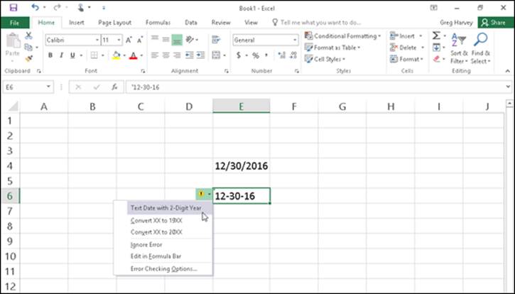
Figure 1-5: Opening the drop-down menu attached to the Number Stored as Text alert.

If you start a cell entry with the equal sign (=) or the at symbol (@) followed by other characters that aren’t part of a formula, Excel displays an error dialog box as soon as you try to complete the data entry. Excel uses the equal sign to indicate the use of a formula, and what you have entered is not a valid formula. The program knows that Lotus 1-2-3 used the @ symbol to indicate the use of a built-in function, and what you have entered is not a valid built-in function. This means that you must preface any data entry beginning with the equal sign and @ symbol that isn’t a valid formula with an apostrophe in order to get it into the cell.

What’s the value?

In a typical spreadsheet, numbers (or numeric data entries) can be as prevalent as the text entries — if not more so. This is because traditionally, spreadsheets were developed to keep financial records, which included plenty of extended item totals, subtotals, averages, percentages, and grand totals. Of course, you can create spreadsheets that are full of numbers that have nothing to do with debits, credits, income statements, invoices, quarterly sales, and dollars and cents.

Number entries that you make in your spreadsheet can be divided into three categories:

· Numbers that you input directly into a cell. (You can do this with the keyboard, your voice if you use the Speech Recognition feature, or even by handwriting if your keyboard is equipped with a writing tablet.)

· Date and time numbers that are also input directly into a cell but are automatically displayed with the default Date and Time number formats and are stored behind the scenes as special date serial and hour decimal numbers.

· Numbers calculated by formulas that you build yourself by using simple arithmetical operators and/or Excel’s sophisticated built-in functions.

Inputting numbers

Numbers that you input directly into the cells of the worksheet — whether they are positive, negative, percentages, or decimal values representing dollars and cents, widgets in stock, workers in the Human Resources department, or potential clients — don’t change unless you specifically change them, either by editing their values or replacing them with other values. This is quite unlike formulas with values that change whenever the worksheet is recalculated and Excel finds that the values upon which they depend have been modified.

When inputting numbers, you can mix the digits 0-9 with the following keyboard characters:

+ - () $ . , %

You use these characters in the numbers you input as follows:

· Preface the digits of the number with a plus sign (+) when you want to explicitly designate the number as positive, as in +(53) to convert negative 53 into positive 53. Excel considers all numbers to be positive unless you designate them as negative.

· Preface the digits of the number with - or enclose them in a pair of parentheses to indicate that the number is a negative number, as in -53 or (53).

· Preface the digits of the number with a dollar sign ($), as in $500, to format the number with the Currency style format as you enter it. (You can also apply this format after it’s entered.)

· Input a period (.) in the digits of the number to indicate the position of the decimal point in the number, as in 500.25. (Note that you don’t have to bother entering trailing zeros after the decimal point because the General number format automatically drops them, even if you type them in.)

· Input commas (,) between the digits of a number to indicate the position of thousands, hundred thousands, millions, billions, and the like, and to assign the Comma style number format to the number, as in 642,153. (You can also have Excel add the commas by assigning the Comma format to the number after you input the number.)

· Append the percent sign (%) to the digits of a number to convert the number into a percentage and assign the Percent number style to it, as in 12%.

The most important thing to remember about the numbers that you input is that they inherit the type of number formatting currently assigned to the cells in which they’re entered. When you first open a blank workbook, the number format appropriately called General (which some have called the equivalent of no number formatting because it doesn’t add any special format characters, such as a constant number of decimal places or thousands separators) is applied to each cell of the worksheet. You can override the General format by adding your own formatting characters as you input the number in a cell or, later, by selecting the cell and then assigning a different number format to it. (See Book II, Chapter 2 for details.)

Dates and times

Excel stores dates and times that you input into a spreadsheet as special values. Dates are stored as serial numbers, and times are stored as decimal fractions. Excel supports two date systems: the 1900 date system used by Excel for Windows (also used by Lotus 1-2-3), which uses January 1, 1900, as serial number 1, and the 1904 system used by Excel for the Macintosh, which uses January 2, 1904, as serial number 1.

If you use Excel on the Windows PCs and Macintosh OS computers in your office, you can switch from the default 1900 date system to the 1904 date system for those worksheets that you create in the Windows version and then transfer to the Macintosh version. To switch to the 1904 date system, click the Advanced tab of the Excel Options dialog box (File  ⇒  Excel Options or Alt+FT) and then select the Use 1904 Date System check box in the When Calculating This Workbook section.

By storing dates as serial numbers representing the number of days that have elapsed from a particular date (January 1, 1900, or January 2, 1904), Excel can perform arithmetic between dates. For example, you can find out how many days there are between February 15, 1949, and February 15, 2016, by entering 2/15/16 in one cell and 2/15/49 in the cell below, and then creating a formula in the cell below that one that subtracts the cell with 2/15/49 from the one containing 2/15/16. Because Excel stores the date 2/15/16 as the serial number 42415 and the date 2/15/49 as the serial number 17944, it can calculate the difference and return the result of 24471 (days, which is equal to 67 years).

When you type a date directly into a formula that performs date arithmetic (as opposed to constructing a formula using references to cells that contain date entries), you must enclose the date in quotation marks. So, for example, if you type the dates in a formula that calculates the number of days between February 15, 1949, and February 15, 2016, in the cell you have to type the following formula:

="2/15/16"-"2/15/49"

Times of the day are stored as decimal numbers that represent the fraction of the 24-hour period starting with 0.0 for 12:00 midnight through 0.999 for 11:59:59 p.m. By storing times as decimal fractions, Excel enables you to perform time calculations such as those that return the elapsed time (in minutes) between any two times of the day.

Inputting dates and times using recognized formats

Although Excel stores dates as serial numbers and times as decimal fractions, luckily you don’t have to use these numbers to enter dates or times of the day into cells of the worksheet. You simply enter dates by using any of the recognized Date number formats that are used by Excel, and you enter times by using any of the recognized Time number formats. Excel then assigns and stores the appropriate serial number or decimal fraction at the same time the program assigns the date or time format that you used for this value. Table 1-1 shows you typical date and time entries that you can use as examples when entering dates and times in the cells of a worksheet.

Table 1-1 Common Ways to Enter Dates and Times

Understanding how Excel treats two-digit years

The only thing that’s a tad bit tricky about inputting dates in a spreadsheet comes in knowing when you have to input all four digits of the year and when you can get away with entering only two. As Table 1-1 shows, if you input the date 1/6/16 in a cell, Excel recognizes the date as 1/6/2016 and not as 1/6/1916. In fact, if you enter the date January 6, 1916, in a spreadsheet, you must enter all four digits of the year (1916).

Here’s how Excel decides whether a year for which you enter only the last two digits belongs to the 20th or 21st century:

· 00 through 29 belong to the 21st century, so Excels interprets 7/30/29 as July 30, 2029.

· 30 through 99 belong to the 20th century, so Excel interprets 7/30/30 as July 30, 1930.

This means that you don’t have to enter the four digits of the year for dates in the years 2000 through 2029, or for dates in the years 1930 through 1999.

Of course, if you can’t remember these cutoffs and are just generally confused about when to enter two digits versus four digits, just go ahead and enter all four digits of the year. Excel never misunderstands which century the date belongs to when you spell out all four digits of the year.

Numeric formulas

Many numeric entries in a typical spreadsheet are not input directly but are returned as the result of a calculation by a formula. The numeric formulas that you build can do anything from simple arithmetic calculations to complex ANOVA statistical analyses. (See Book III for complete coverage of all types of numeric formulas.) Most spreadsheet formulas use numbers that are input into other cells of the worksheet in their calculations. Because these formulas refer to the address of the cell containing the input number rather than the number itself, Excel is able to automatically recalculate the formula and return a new result anytime you change the values in the original cell.

The most important thing to remember about numeric formulas is that their calculated values are displayed in their cells in the worksheet, whereas the contents of the formulas (that indicate how the calculation is done) are displayed on the Formula bar whenever its cell contains the cell cursor. All numbers returned by formulas inherit the nondescript General number format. The only way to get these calculated numbers to appear the way you want them in the worksheet is to select them and apply a new, more appropriate number format to them. (See Book II, Chapter 2for details.)

Data Entry 101

I want to pass on a few basic rules of data entry:

· You must select the cell where you want to make the data entry before you can make the entry in that cell.

· Any entry that you make in a cell that already contains data replaces the original entry.

· Every data entry that you make in any cell must be completed with some sort of action, such as clicking the Enter button on the Formula bar (the button with the check mark that appears when you start entering data), pressing the Enter key, or clicking a new cell before the entry is officially entered in that cell.

I know that the first rule sounds so obvious that it should go without saying, but you’d be surprised how many times you look at the cell where you intend to add new data and then just start entering that data without realizing that you haven’t yet moved the cell cursor to that cell. As a result, the data entry that you’re making is not destined to go into the cell that you intended. In fact, you’re in the process of making the entry in whatever cell currently contains the cell cursor, and if that cell is already occupied, you’re in the process of replacing its entry with the one you meant to go somewhere else!

This is why the third rule is so important: Even if you’re in the process of messing up your spreadsheet by entering data in the wrong cell (and, if that cell is occupied, you’re destroying a perfectly good entry), you haven’t done it until you take the action that completes the entry (such as clicking the Enter button on the Formula bar or pressing the Enter key). This means that you can recover simply by clicking the Cancel button on the Formula bar or by pressing the Escape key on your keyboard. As soon as you do that, the errant data entry disappears from the Formula bar (and the original data entry — if it exists — returns), and you’re then free to move the cell cursor to the desired cell and redo the entry there.

Data entry keyboard style

The only trick to entering data from the keyboard is to figure out the most efficient way to complete the entry in the current cell (and Excel gives you many choices in this regard). You can, of course, complete any data entry by selecting the Enter button on the Formula bar (presumably this is what Microsoft intended; otherwise, why have the button?), but clicking this button is not at all efficient when the mouse pointer isn’t close to it.

You should know of another potential drawback to clicking the Enter button on the Formula bar to complete an entry: When you do this, Excel doesn’t move the cell cursor but keeps it right in the cell with the new data entry. This means that you still have to move the cell cursor before you can safely make your next data entry. You’re better off pressing the Enter key because doing this not only completes the entry in the cell, but also moves the cell cursor down to the cell in the next row.

Of course, pressing the Enter key is efficient only if you’re doing the data entry for a table or list down each row across the succeeding columns. If you want to enter the data across each column of the table or list down succeeding rows, pressing Enter doesn’t work to your advantage. Instead, you’d be better off pressing the → key or the Tab key to complete each entry (at least until you get to the cell in the last column of the table) because pressing these keys completes the entry and moves the cell cursor to the next cell on the right.

Take a look at Table 1-2 to get an idea of the keys that you commonly use to complete data entries. Keep in mind, however, that any key combination that moves the cell cursor (see Table 1-1 in Book I, Chapter 1, for a review of these keystrokes) also completes the data entry that you’re making, as does clicking another cell in the worksheet.

Table 1-2 Keys Used in Completing Data Entry

If you have more than one cell selected (see Book II, Chapter 2 for more on this) and then press Ctrl+Enter to complete the data entry that you’re making in the active cell of this selected range, Excel simultaneously enters that data entry into all the cells in the selection. You can use this technique to enter a single label or value in many places in a worksheet at one time.

If you have more than one worksheet selected (see Book II, Chapter 4) at the time that you make an entry in the current cell, Excel makes that entry in the corresponding cells of all the selected worksheets. For example, if you enter the heading Cost Analysis in cell C3 of Sheet1 when Sheet1 through Sheet3 are selected, Excel enters Cost Analysis in cell C3 of Sheet2 and Sheet3 as well.

Doing data entry with the Touch keyboard

If you’re running Excel 2016 on a touchscreen device that lacks any kind of physical keyboard, such as a Surface 3 tablet without the optional Type Cover, you need to open the Touch keyboard and use it to input your spreadsheet data. To open the Touch keyboard, simply tap the Touch Keyboard button that appears on the right side of the Windows 7, 8, or 10 taskbar. Doing this displays the Touch keyboard docked at the bottom of the Excel program window.

To undock the Touch keyboard beneath the Excel 2016 program window, click the Dock/Undock button that appears to the immediate left of the Close button in the upper-right corner of the keyboard. Figure 1-6 shows you how your touchscreen looks after undocking the Windows 10 Touch keyboard and dragging it up away from the Excel status bar.

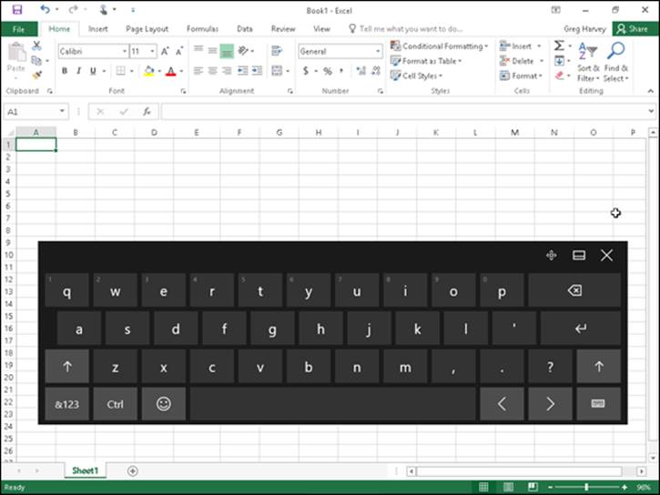
Figure 1-6: A Windows 10 touchscreen after displaying and undocking the Touch keyboard so it floats in the middle of the Excel 2016 program window.

As shown in this figure, when undocked, the Windows 10 Touch keyboard remains completely separate from the Excel program window so that you can reposition it so that you still have access to most of the cells in the current worksheet when doing your data entry. The Windows 10 Touch keyboard is limited mostly to letter keys above a spacebar with a few punctuation symbols (apostrophe, comma, period, and question mark). This keyboard also sports the following special keys:

· Backspace key (marked with the x in the shape pointing left) to delete characters to the immediate left when entering or editing a cell entry

· Enter key (with the bent arrow) to complete an entry in the current cell and move the cursor down one row in the same column

· Shift keys (with arrows pointing upward) to enter capital letters in a cell entry

· Numeric key (with &123) to switch to the Touch keyboard so that it displays a numeric keyboard with a Tab key and extensive punctuation used in entering numeric data in a cell (tap the &123 key a second time to return to the standard QWERTY letter arrangement)

· Ctrl key to run macros to which you’ve assigned letter keys (see Book VIII, Chapter 1 for details) or to combine with the left arrow or right arrow key to jump the cursor to the cell in the last and first column of the current row, respectively

· Emoticon key (with that awful smiley face icon) to switch to a bunch of emoticons that you can enter into a cell entry (tap the Emoticon key a second time to return to standard QWERTY letter arrangement)

· Left arrow (with the < symbol) to move the cell cursor one cell to the immediate right and complete any cell entry in progress

· Right arrow (with the > symbol) to move the cell cursor one cell to the immediate left and complete any cell entry in progress

When you finish entering your worksheet data with your Windows Touch keyboard, you can close it and return to the normal full screen view of the Excel program window by tapping the Close button.

The Windows Touch keyboard supports a split-keyboard arrangement that enables you to see more of the cells in your worksheet as you enter your text and numbers in the worksheet from separated banks of keys on the left and right side of the worksheet area. To switch to this arrangement, tap the Keyboard button in the very lower-right corner of the Touch keyboard and then tap the second-from-the-left icon with the picture of a keyboard with space in the middle from the pop-up menu that appears. Excel then displays the split-Touch keyboard with a version of the ten-key keypad in the middle of the keyboard and the QWERTY letter keys separated into a left and right bank. You can also switch to an Inking keyboard (the icon second from the right with a stylus sticking out of it) where you can make cell entries by writing your entries in the keyboard area with your stylus and then inserting them into the worksheet by tapping its Insert button.

You AutoComplete this for me

Excel automatically makes use of a feature called AutoComplete, which attempts to automate completely textual data entries (that is, entries that don’t mix text and numbers). AutoComplete works this way: If you start a new text entry that begins with the same letter or letters as an entry that you’ve made recently in the same region of the worksheet, Excel completes the new text entry with the characters from the previous text entry that began with those letters.

For example, if you type the spreadsheet title Sales Invoice in cell A1 of a new worksheet and then, after completing the entry by pressing the ↓, start entering the table title Summary in cell A2, as soon as you type S in cell A2, Excel completes the new text entry so that it also states Sales Invoice by adding the letters ales Invoice.

When the AutoComplete feature completes the new text entry, the letters that it adds to the initial letter or letters that you type are automatically selected (indicated by highlighting). This way, if you don’t want to repeat the original text entry in the new cell, you can replace the characters that Excel adds just by typing the next letter in the new (and different) entry. In the previous example, in which Sales Invoice was repeated in the cell where you want to input Summary, the ales Invoice text appended to the S that you type disappears the moment you type u in Summary.

Note that when you have two different entries that begin with the same first letter but have different second letters, typing the second letter of one entry causes Excel to complete the typing of that entry, leaving you free to insert its text in the cell by pressing the Enter key or using any of the other methods for completing a cell entry.

To make use of automatic text completion rather than override it as in the previous example, simply press a key (such as Enter, Tab, or an arrow key), click the Enter button on the Formula bar, or click another cell to complete the completed input in that cell. For example, say you’re building a sales table in which you’re inputting sales for three different account representatives — George, Jean, and Alice. After entering each name manually in the appropriate row of the Account Representative column, you need to type in only their first initial (G to get George, J to get Jean, and A to get Alice) in subsequent cells and then press the ↓ or Enter key to move down to the next row of that column. Of course, in a case like this, AutoComplete is more like automatic typing, and it makes filling in the Account Representative names for this table extremely quick and easy.

If the AutoComplete feature starts to bug you when building a particular spreadsheet, you can temporarily turn it off; simply click the Enable AutoComplete for Cell Values check box in the Editing Options section, and remove the check mark on the Advanced tab of the Excel Options dialog box (File  ⇒  Options or Alt+FTA). Note that disabling AutoComplete in this manner also disables the Flash Fill feature as well. (See “Flash Fill to the rescue” later in this chapter for details.)

You AutoCorrect this right now!

Along with AutoComplete, Excel has an AutoCorrect feature that automatically fixes certain typos that you make in the text entries as soon as you complete them. For example, if you forget to capitalize a day of the week, AutoCorrect does this for you (turning friday into Friday in a cell as soon as you complete the entry). Likewise, if you mistakenly enter a word with two initial capital letters, AutoCorrect automatically lowercases the second capital letter (so that QUarter typed into a cell becomes Quarter upon completion of the cell entry).

In addition to these types of obvious capitalization errors, AutoCorrect also automatically takes care of common typos, such as changing hsi to his (an obvious transposition of two letters) or inthe to in the (an obvious case of a missing space between letters). In addition to the errors already recognized by AutoCorrect, you can add your own particular mistakes to the list of automatic replacements.

To do this, open the AutoCorrect dialog box and then add your own replacements in the Replace and With text boxes located on the AutoCorrect tab, shown in Figure 1-7. Here’s how:

1. Select File  ⇒  Options and then click the Proofing tab (Alt+FTP) followed by the AutoCorrect Options button.

The AutoCorrect dialog box opens for your language, such as English (U.S.).

2. If the AutoCorrect options aren’t already displayed in the dialog box, click the AutoCorrect tab to display them.

3. Click the Replace text box and then enter the typo exactly as you usually make it.

4. Click the With text box and enter the replacement that AutoCorrect should make (with no typos in it, please!).

Check the typo that you’ve entered in the Replace text box and the replacement that you’ve entered in the With text box. If everything checks out, go on to Step 5.

5. Click the Add button to add your new AutoCorrect replacement to the list of automated replacements.

6. Click the OK button to close the AutoCorrect dialog box.

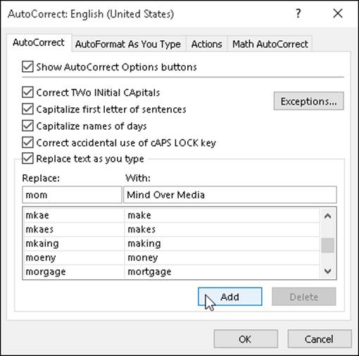
Figure 1-7: You can add your own automated replacements to the AutoCorrect tab.

You can use the AutoCorrect feature to automatically replace favorite abbreviations with full text, as well as to clean up all your personal typing mistakes. For example, if you have a client with the name Great Lakes Securities, and you enter this client’s name in countless spreadsheets that you create, you can make an AutoCorrect entry so that Excel automatically replaces the abbreviation gls with Great Lakes Securities. Of course, after you use AutoCorrect to enter Great Lakes Securities in your first cell by typing gls, the AutoComplete feature kicks in, so the next time you type the g of gls to enter the client’s name in another cell, it fills in the rest of the name, leaving you with nothing to do but complete the entry.

Keep in mind that AutoCorrect is not a replacement for Excel’s spelling checker. You should still spell check your spreadsheet before sending it out because the spelling checker finds all those uncommon typos that haven’t been automatically corrected for you. (See Book II,Chapter 3 for details.)

Constraining data entry to a cell range

One of the most efficient ways to enter data into a new table in your spreadsheet is to preselect the empty cells where the data entries need to be made and then enter the data into the selected range. Of course, this trick only works if you know ahead of time how many columns and rows the new table requires.

The reason that preselecting the cells works so well is that doing this constrains the cell cursor to that range, provided that you press only the keystrokes shown in Table 1-3. This means that if you’re using the Enter key to move down the column as you enter data, Excel automatically positions the cell cursor at the beginning of the next column as soon as you complete the last entry in that column. Likewise, when using the Tab key to move the cell cursor across a row as you enter data, Excel automatically positions the cell cursor at the beginning of the next row in the table as soon as you complete the last entry in that row.

Table 1-3 Keystrokes for Moving Within a Selection

That way you don’t have to concentrate on repositioning the cell cursor at all when entering the table data; you can keep your attention on the printed copy from which you’re taking the data.

You can’t very well use this preselection method on data lists because they’re usually open-ended affairs to which you continually append new rows of data. The most efficient way to add new data to a new or existing data list is to format it as a table. (See Book II, Chapter 2.)

Getting Excel to put in the decimal point

Of course, if your keyboard has a ten-key entry pad, you’ll want to use it rather than the numbers on the top row of the keyboard to make your numeric entries in the spreadsheet. (Make sure that the Num Lock key is engaged, or you’ll end up moving the cell cursor rather than entering numbers.) If you have a lot of decimal numbers (suppose that you’re building a financial spreadsheet with loads of dollars and cents entries), you may also want to use Excel’s Fixed Decimal Places feature so that Excel places a decimal point in all the numbers that you enter in the worksheet.

To turn on this feature, click the Automatically Insert a Decimal Point check box in the Editing Options section of the Advanced tab of the Excel Options dialog box (Alt+FTA) to put a check mark in it. When you do this, the Places text box immediately below it determines the number of decimal places that the program is to add to each number entry. You can then specify the number of places by changing its value (2 is, of course, the default) either by entering a new value or selecting one with its spinner buttons.

After turning on the Automatically Insert a Decimal Point option, Excel adds a decimal point to the number of places that you specified to every numeric data entry that you make at the time you complete its entry. For example, if you type the digits 56789 in a cell, Excel changes this to 567.89 at the time you complete the entry.

Note that when this feature is turned on and you want to enter a number without a decimal point, you need to type a period at the end of the value. For example, if you want to enter the number 56789 in a cell and not have Excel change it to 567.89, you need to type

56789.

Ending the number in a period prevents Excel from adding its own decimal point to the value when Fixed Decimal Places is turned on. Of course, you need to turn this feature off after you finish making the group of entries that require the same number of decimal places. To do this, deselect the Automatically Insert a Decimal Point check box on the Advanced tab of the Excel Options dialog box (Alt+FTA).

You AutoFill it in

Few Excel features are more helpful than the AutoFill feature, which enables you to fill out a series of entries in a data table or list — all by entering only the first item in the series in the spreadsheet. You can sometimes use the AutoFill feature to quickly input row and column headings for a new data table or to number the records in a data list. For example, when you need a row of column headings that list the 12 months for a sales table, you can enter January or Jan. in the first column and then have AutoFill input the other 11 months for you in the cells in columns to the right. Likewise, when you need to create a column of row headings at the start of a table with successive part numbers that start at L505-120 and proceed to L505-128, you enter L505-120 in the first row and then use AutoFill to copy the part numbers down to L505-128 in the cells below.

The key to using AutoFill is the Fill handle, which is the small black square that appears in the lower-right corner of whatever cell contains the cell cursor. When you position the mouse or Touch pointer on the Fill handle, it changes from the normal thick, white-cross pointer to a thin, black-cross pointer. This change in shape is your signal that when you drag the Fill handle in a single direction, either down or to the right, Excel will either copy the current cell entry to all the cells that you select or use it as the first entry in a consecutive series, whose successive entries are then automatically entered in the selected cells.

Note that you can immediately tell whether Excel will simply copy the cell entry or use it as the first in a series to fill out by the ScreenTips that appear to the right of the mouse pointer. As you drag through subsequent cells, the ScreenTip indicates which entry will be made if you release the mouse button (or remove your finger or stylus from a touchscreen) at that point. If the ScreenTip shows the same entry as you drag, you know Excel didn’t recognize the entry as part of a consecutive series and is copying the entry verbatim. If, instead, the ScreenTips continue to change as you drag through cells showing you successive entries for the series, you know that Excel has recognized the original entry as part of a consecutive series.

Figures 1-8 and 1-9 illustrate how AutoFill works. In Figure 1-8, I entered January as the first column heading in cell B2 (using the Enter button on the Formula bar so as to keep the cell cursor in B2, ready for AutoFill). Next, I positioned the mouse pointer on the AutoFill handle in the lower-right corner of B2 before dragging the Fill handle to the right until I reached cell G2 (and the ScreenTip stated June).

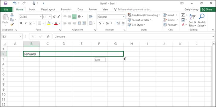
Figure 1-8: Dragging the Fill handle to fill in a series with the first six months of the year.

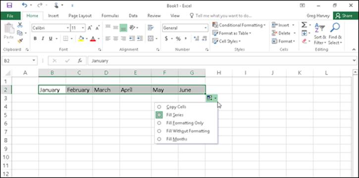
Figure 1-9: The series of monthly column headings with the AutoFill Options drop-down menu.

Figure 1-9 shows the series that was entered in the cell range B2:G2 when I released the mouse button with cell G2 selected. For this figure, I also clicked the drop-down button attached to the Auto Fill Options button that automatically appears whenever you use the Fill handle to copy entries or fill in a series to show you the items on this drop-down menu. This menu contains a Copy Cells option button that enables you to override Excel’s decision to fill in the series and have it copy the original entry (January, in this case) to all the selected cells.

Note that you can also override Excel’s natural decision to fill in a series or copy an entry before you drag the Fill handle. To do so, simply hold down the Ctrl key (which adds a tiny plus sign to the upper-right corner of the Fill handle). Continue to depress the Ctrl key as you drag the Fill handle and notice that the ScreenTip now shows that Excel is no longer filling in the series or copying the entry as expected.

When you need to consecutively number the cells in a range, use the Ctrl key to override Excel’s natural tendency to copy the number to all the cells you select. For example, if you want to number rows of a list, enter the starting number (1 or 100, it doesn’t matter) in the first row, then press Ctrl to have Excel fill in the rest of the numbers for successive rows in the list (2, 3, 4, and the like, or 102, 103, 104, and so on). If you forget to hold down the Ctrl key and end up with a whole range of cells with the same starting number, click the Auto Fill Options drop-down button and then click the Fill Series option button to rectify the mistake by converting the copied numbers to a consecutively numbered series.

When using AutoFill to fill in a data series, you don’t have to start with the first entry in that particular series. For example, if you want to enter a row of column headings with the last six months of the year (June through December), you enter June first and then drag down or to the right until the mouse pointer selects the cell where you enter December (indicated by the December ScreenTip). Note also that you can reverse-enter a data series by dragging the Fill handle up or left. In the June-to-December column headings example, if you drag up or left, Excel enters June to January in reverse order.

Keep in mind that you can also use AutoFill to copy an original formula across rows and down columns of data tables and lists. When you drag the Fill handle in a cell that contains a formula, Excel automatically adjusts its cell references to suit the new row or column position of each copy. (See Book III, Chapter 1 for details on copying formulas with AutoFill.)

AutoFill on a Touchscreen

To fill out a data series using your finger or stylus when using Excel on a touchscreen tablet without access to a mouse or touchpad, you use the AutoFill button that appears on the touchscreen mini-toolbar as follows:

1. Tap the cell containing the initial value in the series you want AutoFill to extend.

Excel selects the cell and displays selection handles (with circles) in the upper-left and lower-right corners.

2. Tap and hold the cell until the mini-toolbar appears.

When summoned by touch, the mini-toolbar appears as a single row of command buttons, Paste to AutoFill, terminated by a Show Context Menu button (with a black triangle pointing downward).

3. Tap the AutoFill button on the mini-toolbar.

Excel closes the mini-toolbar and adds an AutoFill button to the currently selected cell (with a blue downward-pointing arrow in the square).

4. Drag the AutoFill button through the blank cells in the same column or row into which the data series sequence is to be filled.

When you release your finger or stylus after selecting the last blank cell to be filled, Excel fills out the data series in the selected range.

AutoFill via the Fill button on the Ribbon

Instead of using the Fill handle or AutoFill button on a touchscreen’s mini-toolbar, you can also fill out a series using the Fill button on the Excel 2016 Ribbon. To use the Fill button on the Home tab of the Ribbon to accomplish your AutoFill operations, you follow these steps:

1. Enter the first entry (or entries) upon which the series is to be based in the first cell(s) to hold the new data series in your worksheet.

2. Select the cell range where the series is to be created, across a row or down a column, being sure to include the cell with the initial entry or entries in this range.

3. Select the Fill button on the Home tab and choose Series from its drop-down menu or press Alt+HFIS.

The Fill button is located in the Editing group right below the AutoSum button (the one with the Greek sigma). When you select the Series option, Excel opens the Series dialog box.

4. Click the AutoFill option button in the Type column followed by the OK button in the Series dialog box.

Excel enters a series of data based on the initial value(s) in your selected cell range just as though you’d selected the range with the fill handle.

Note that the Series dialog box contains a bunch of options that you can use to further refine and control the data series that Excel creates. In a linear data series, if you want the series to increment more than one step value at a time, you can increase it in the Step Value text box. Likewise, if you want your linear or AutoFill series to stop when it reaches a particular value, you enter that into the Stop Value text box.

When you’re entering a series of dates with AutoFill that increment on anything other than the day, remember the Date Unit options in the Series dialog box enable you to specify other parts of the initial date to increment in the series. Your choices include Weekday, Month, or Year.

Filling series with increments other than one

Normally, when you drag the Fill handle to fill in a series of data entries, Excel increases or decreases each entry in the series by a single unit (a day, month, hour, or whatever). You can, however, get AutoFill to fill out a series of data entries that uses some other increment, such as every other day, every third month, or every hour-and-a-half.

Figure 1-10 illustrates a number of series all created with AutoFill that use increments other than one unit. The first example in row 2 shows a series of different times all 45 minutes apart, starting with 8:00 a.m. in cell A3 and extending to 2:00 p.m. in cell I3. The second example in row 4 contains a series of weekdays consisting of every other day of the week, starting on Monday in cell A4 and extending to Saturday in cell G4. The third example in row 6 shows a series of numbers, each of which increases by 15, that starts with 35 in cell A6 and increases to 155 in cell I6. The last example in row 8 shows a series with every other month, starting with Jan. in cell A8 and ending with Nov. in cell F8.

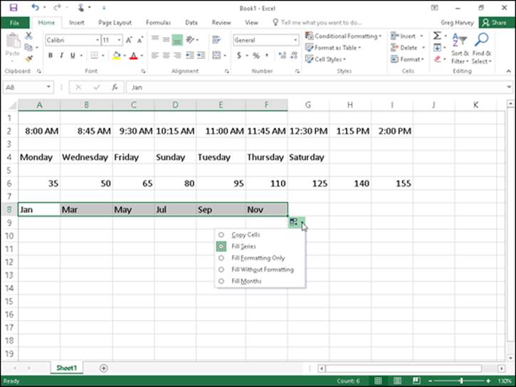
Figure 1-10: Various series created with AutoFill by using different increments.

To create a series that uses an increment other than one unit, follow these four general steps:

1. Enter the first two entries in the series in consecutive cells above one another in a column or side by side in a row.

Enter the entries one above the other when you intend to drag the Fill handle down the column to extend the series. Enter them side by side when you intend to drag the Fill handle to the right across the row.

2. Position the cell pointer in the cell with the first entry in the series, and drag through the second entry.

Both entries must be selected (indicated by being enclosed within the expanded cell cursor) before you use the Fill handle to extend the series. Excel analyzes the difference between the two entries and uses its increment in filling out the data series.

3. Drag the Fill handle down the column or across the row to extend the series by using the increment other than one unit.

Check the ScreenTips to make sure that Excel is using the correct increment in filling out your data series.

4. Release the mouse button when you reach the desired end of the series (indicated by the entry shown in the ScreenTip appearing next to the black-cross mouse pointer).

Creating custom AutoFill lists

Just as you can use AutoFill to fill out a series with increments different from one unit, you can also get it to fill out custom lists of your own design. For example, suppose that you often have to enter a standard series of city locations as the column or row headings in new spreadsheets that you build. Instead of copying the list of cities from one workbook to another, you can create a custom list containing all the cities in the order in which they normally appear in your spreadsheets. After you create a custom list in Excel, you can then enter all or part of the entries in the series simply by entering the first item in a cell and then using the Fill handle to extend out the series either down a column or across a row.

To create a custom series, you can either enter the list of entries in the custom series in successive cells of a worksheet before you open the Custom Lists dialog box, or you can type the sequence of entries for the custom series in the List Entries list box located on the right side of the Custom Lists tab in this dialog box, as shown in Figure 1-11.

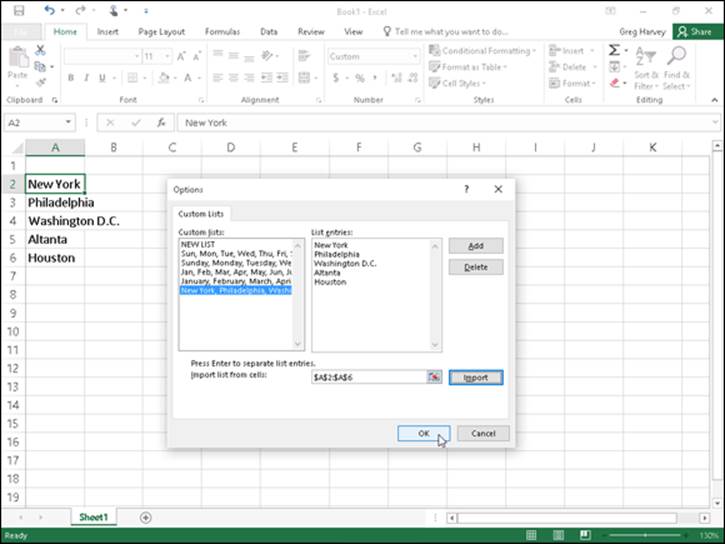
Figure 1-11: Creating a custom list of cities for AutoFill.

If you already have the data series for your custom list entered in a range of cells somewhere in a worksheet, follow these steps to create the custom list:

1. Click the cell with the first entry in the custom series and then drag the mouse or Touch pointer through the range until all the cells with entries are selected.

The expanded cell cursor should now include all the cells with entries for the custom list.

2. Select File  ⇒  Options  ⇒  Advanced (Alt+FTA) and then scroll down and click the Edit Custom Lists button located in the General section.

The Custom Lists dialog box opens with its Custom Lists tab, where you now should check the accuracy of the cell range listed in the Import List from Cells text box. (The range in this box lists the first cell and last cell in the current selected range separated by a colon — you can ignore the dollar signs following each part of the cell address.) To check that the cell range listed in the Import List from Cells text box includes all the entries for the custom list, click the Collapse Dialog Box button, located to the right of the Import List from Cells text box. When you click this button, Excel collapses the Custom Lists dialog box down to the Import List from Cells text box and puts a marquee (the so-called marching ants) around the cell range.

If this marquee includes all the entries for your custom list, you can expand the Custom Lists dialog box by clicking the Expand Dialog box button (which replaces the Collapse Dialog Box button) and proceed to Step 3. If this marquee doesn’t include all the entries, click the cell with the first entry and then drag through until all the other cells are enclosed in the marquee. Then, click the Expand Dialog box button and go to Step 3.

3. Click the Import button to add the entries in the selected cell range to the List Entries box on the right and to the Custom Lists box on the left side of the Custom Lists tab.

As soon as you click the Import button, Excel adds the data entries in the selected cell range to both the List Entries and the Custom Lists boxes.

4. Select the OK button twice, the first time to close the Custom Lists dialog box and the second to close the Excel Options dialog box.

If you don’t have the entries for your custom list entered anywhere in the worksheet, you have to follow the second and third steps listed previously and then take these three additional steps instead:

1. Click the List Entries box and then type each of the entries for the custom list in the order in which they are to be entered in successive cells of a worksheet.

Press the Enter key after typing each entry for the custom list so that each entry appears on its own line in the List Entries box, or separate each entry with a comma.

2. Click the Add button to add the entries that you’ve typed into the List Entries box on the right to the Custom Lists box, located on the left side of the Custom Lists tab.

Note that when Excel adds the custom list that you just typed to the Custom Lists box, it automatically adds commas between each entry in the list — even if you pressed the Enter key after making each entry. It also automatically separates each entry on a separate line in the List Entries box — even if you separated them with commas instead of carriage returns.

3. Click the OK button twice to close both the Custom Lists box and Excel Options dialog box.

After you’ve created a custom list by using one of these two methods, you can fill in the entire data series by entering the first entry of the list in a cell and then dragging the Fill handle to fill in the rest of the entries. If you ever decide that you no longer need a custom list that you’ve created, you can delete it by clicking the list in the Custom Lists box in the Custom Lists dialog box and then clicking the Delete button. Excel then displays an alert box indicating that the list will be permanently deleted when you click OK. Note that you can’t delete any of the built-in lists that appear in this list box when you first open the Custom Lists dialog box.

Keep in mind that you can also fill in any part of the series by simply entering any one of the entries in the custom list and then dragging the Fill handle in the appropriate direction (down and to the right to enter succeeding entries in the list or up and to the left to enter preceding entries).

Flash Fill to the rescue

Excel 2016’s handy Flash Fill feature gives you the ability to take a part of the data entered into one column of a worksheet table and enter just that data in a new table column using only a few keystrokes. The series of entries appear in the new column, literally in a flash (thus, the nameFlash Fill), the moment Excel detects a pattern in your initial data entry that enables it to figure out the data you want to copy. The beauty is that all this happens without the need for you to construct or copy any kind of formula.

The best way to understand Flash Fill is to see it in action. Figure 1-12 contains a new data table consisting of four columns. The first column already contains the full names of clients (first, middle, and last). The second, third, and fourth columns need to have just the first, middle, and surnames, respectively, entered into them (so that particular parts of the clients’ names can be used in the greetings of form e-mails and letters as in, “Hello Keith,” or “Dear Mr. Harper,”).

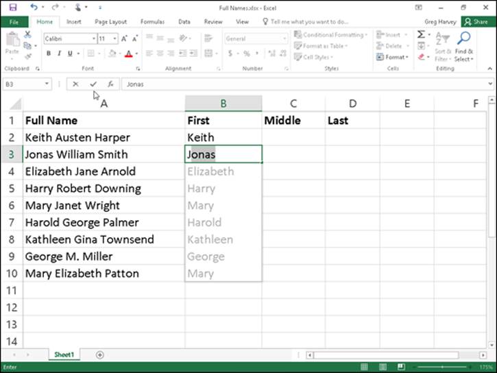
Figure 1-12: New data table containing full names that need to be split up in separate columns with Flash Fill.

Rather than manually entering the first, middle, or last names in the respective columns (or attempting to copy the entire client name from column A and then editing out the parts not needed in the First Name, Middle Name, and Last Name columns), you can use Flash Fill to quickly and effectively do the job. And here’s how you do it:

1. Type Keith in cell B2 and complete the entry with the ↓ or Enter key.

When you complete this entry with the ↓ key or Enter key on your keyboard, Excel moves the cell pointer to cell B3, where you have to type only the first letter of the next name for Flash Fill to get the picture.

2. In Cell B3, type only J, the first letter of Jonas, the second client’s first name.

Flash Fill immediately does an AutoFill type maneuver by suggesting the rest of the second client’s first name, Jonas, as the text to enter in this cell. At the same time, Flash Fill suggests entering all the remaining first names from the full names in column A in column B. (See Figure 1-12.)

3. Complete the entry of Jonas in cell B3 by clicking the Enter button or pressing an arrow key.

The moment you complete the data entry in cell B3, the First Name column is done: Excel enters all the other first names in column B at the same time!

To complete this example name table by entering the middle and last names in columns C and D, respectively, you simply repeat these steps in those columns. You enter the first middle name, Austen, from cell A2 in cell C2 and then type W in cell C3. Complete the entry in cell C3 and the middle name entries in that column are done. Likewise, you enter the first last name, Harper, from cell A2 in cell D2 and then type S in cell D3. Complete the entry in cell D3, and the last name entries for column D are done, finishing the entire data table.

By my count, completing the data entry in this Client Name table required me to make a total of 26 keystrokes, 20 of which were for typing in the first, middle, and last name of the first client along with the initial letters of the first, middle, and last name of the second client and the other six to complete these entries. If Column A of this Client Name table contains the full names of hundreds or even thousands of clients, this 26 keystrokes is insignificant compared to the number that would be required to manually enter their first, middle, and last names in their separate First Name, Middle Name, and Last Name columns or even to edit down copies of the full names in each of them.

Keep in mind that Flash Fill works perfectly at extracting parts of longer data entries in a column provided that all the entries follow the same pattern and use same type of separators (spaces, commas, dashes, and the like). For example, in Figure 1-11, there’s an anomaly in the full name entries in cell A9 where only the middle initial with a period is entered instead of the full middle. In this case, Flash Fill simply enters M in cell C9, and you have to manually edit its entry to add the necessary period. Also, remember that Flash Fill’s usefulness isn’t restricted to all-text entries as in my example Client Name table. It can also extract parts of entries that mix text and numbers, such as ID numbers (AJ-1234, RW-8007, and so forth).

Limiting data entry with Data Validation

The Data Validation feature in Excel can be a real timesaver when you’re doing repetitive data entry, and can also go a long way in preventing incorrect entries in your spreadsheets. When you use Data Validation in a cell, you indicate what type of data entry is allowed in the cell. As part of restricting a data entry to a number (which can be a whole number, decimal, date, or time), you also specify the permissible values for that type of number (a whole number between 10 and 100 or a date between January 1, 2016, and December 31, 2016, for example).

When you restrict the data entry to text, you can specify the range of the minimum and maximum text length (in characters) or, even better, a list of permissible text entries that you can select from a pop-up menu (opened by clicking a pop-up button that appears to the right of the cell whenever it contains the cell cursor).

When using Data Validation to restrict the type of data entry and its range of acceptable values in a cell, you can also specify an input message that is automatically displayed next to the cell when you select it and/or an error alert message that is displayed if you try to input the wrong type of entry or a number outside the permissible range.

To use the Data Validation feature, put the cell cursor in the cell where you want to restrict the type of data entry that you can make there, and then click the Data Validation button on the Data tab of the Ribbon (or press Alt+AVV). The Data Validation dialog box opens with the Settings tab selected (similar to the one shown in Figure 1-13).

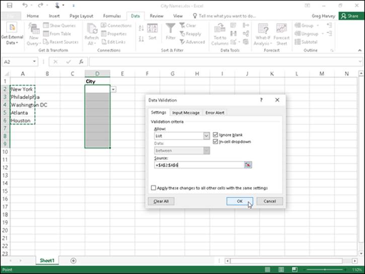
Figure 1-13: Creating a custom drop-down list in the Data Validation dialog box.

You then click the drop-down button attached to the Allow drop-down list box and select among the following items:

· Any Value to remove any previous restrictions thereby canceling data validation and once again enabling the user to enter anything he wishes into the cell

· Whole Number to restrict the entry to a whole number that falls within a certain range or adheres to particular parameters that you specify

· Decimal to restrict the entry to a decimal number that falls within a certain range or adheres to particular parameters that you specify

· List to restrict the entry to one of several text entries that you specify, which you can select from a pop-up menu that’s displayed by clicking a pop-up button that appears to the right of the cell whenever it contains the cell cursor

· Date to restrict the entry to a date that falls within a certain range or on or before a particular date

· Time to restrict the entry to a time that falls within a certain range or on or before a particular time of the day

· Text Length to restrict a text entry so that its length in characters doesn’t fall below or go above a certain number or falls within a range that you specify

· Custom to restrict the entry to the parameters specified by a particular formula entered in another cell of the worksheet

To specify an input message after selecting all the items on the Settings tab, click the Input Message tab of the Data Validation dialog box, where you enter a short title for the input message (such as List Entry) in the Title text box, and then enter the text of your message in the Input Message list box below.

To specify an alert message, click the Error Alert tab of the Data Validation dialog box, where you can select the kind of warning from the Style drop-down list: Stop (the default, which uses a red button with a cross in it), Warning (which uses a yellow triangle with an exclamation point in it), or Information (which uses a balloon with a blue I in it). After selecting the type of alert, you then enter the title for its dialog box in its Title text box and enter the text of the alert message in the Error Message list box.

To apply the restriction you’re defining in the Data Validation dialog box to all the other cells that are formatted the same way as in a cell range formatted as a table (see Book II, Chapter 2 for details), click the Apply These Changes to All Other Cells with the Same Settings check box before you click OK. To copy the restriction to a range that is not formatted as a table, use the Data Validation feature to set up the type of entry and permitted range in the first cell and then use the Fill handle to copy that cell’s Data Validation settings to subsequent cells in the same column or row.

By far, the most popular use of the Data Validation feature is to create a drop-down menu from which you or someone who uses your spreadsheet can select the appropriate data entry. Figures 1-13 and 1-14 illustrate this type of usage.

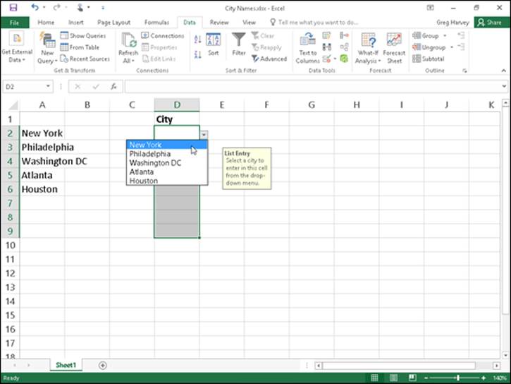
Figure 1-14: Selecting a city from the custom drop-down list.

As Figure 1-13 shows, on the Settings tab of the Data Validation dialog box, I chose List from the Allow drop-down list box and then in the Source text box, I designated the cell range A2:A6, which just happens to contain the list of allowable entries. (You can type them in the Source text box separated by commas if the list doesn’t already exist someplace on the worksheet.) Notice in this figure that, as soon as you select List in the Allow combo box, a check box appears. Keep this check box selected because it tells Excel to create a drop-down list (or pop-up menu, as it’s also called) containing only the entries specified in the Source text box.

Figure 1-14 shows you what happens in the spreadsheet after you close the Data Validation dialog box. Here, you see the pop-up menu (with a list of cities taken from the cell range A2:A6) as it appears when you click the cell’s new pop-up button. In this figure, you can also see the input List Entry message box that I created for this cell by using the options on the Input Message tab of the Data Validation dialog box. Note that you can reposition this message box (officially known as a comment box) so that it’s close to the cell but doesn’t get in the way of selecting an entry — simply drag the comment box with the mouse pointer.

Figure 1-15 demonstrates what happens if you try to input an entry that isn’t on the drop-down list. For this figure, I deliberately disregarded the input instructions and typed Boston as the location. As soon as I clicked the Enter button on the Formula bar, the custom alert dialog box (which I named Not On the List!) appears. I created this alert dialog box by using the options located on the Error Alert tab of the Data Validation dialog box.

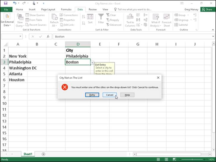
Figure 1-15: Getting an error message after trying to input a city that’s not on the list.

To find cells to which Data Validation has been applied, open the Go To dialog box (Ctrl+G or F5), and then click the Special button and click the Data Validation option button in the Go To Special dialog box. Click the Same option button under Data Validation to have Excel go to the next cell that uses the same Data Validation settings as the active cell. Leave the All option button under Data Validation selected to go to the next cell that uses any kind of Data Validation setting.

To get rid of Data Validation settings assigned to a particular cell or cell range, select the cell or range, open the Data Validation dialog box (Alt+AVV), and then click the Clear All button before you click OK.

Although Data Validation is most often used to restrict new data entries in a spreadsheet, you can also use it to quickly identify values that are outside desired parameters in ranges of existing numeric data entries — see Book II, Chapter 3 for details.

Saving the Data

One of the most important tasks you ever perform when building your spreadsheet is saving your work! Excel offers three different ways to invoke the Save command:

· Select the Save button on the Quick Access toolbar (the one with the disk icon).

· Press Ctrl+S or F12.

· Select File  ⇒  Save.

To encourage frequent saving on your part, Excel provides you with a Save button on the Quick Access toolbar (the one with the picture of a floppy disk, the very first on the toolbar). You don’t even have to take the time and trouble to choose the Save command from the File pull-down menu or even press Ctrl+S; you can simply click this button whenever you want to save new work on disk.

When you click the Save button, press Ctrl+S, or click File  ⇒  Save for the first time, Excel displays the Save As screen in the Backstage view similar to the one shown in Figure 1-16. By default, Excel 2016 selects the Documents folder on your OneDrive as the place to which to save the new workbook.

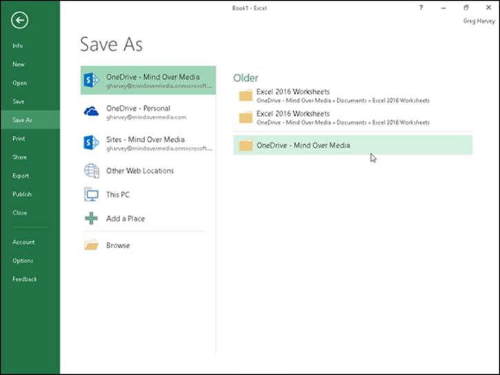
Figure 1-16: Specifying the place to save a new workbook file on the Save As screen.

What’s up with the OneDrive?

You’ve undoubtedly heard of the cloud (sometimes called the “almighty Cloud”), but your understanding of it may yet be as nebulous as its name. OneDrive (once known as SkyDrive) is the current name that Microsoft’s storage space in the cloud that it lends to its users with a Windows acount The great thing about saving a workbook file in a folder on your OneDrive is that you then can open it for further editing and printing from any device running Excel 2016 that has Internet access. For example, if you save a workbook file that you create in Excel on your office desktop computer, you can then open it for more editing on your laptop at home or even your Windows tablet or smartphone at the local coffee shop. For more information on OneDrive and to set it up on your computer, open the Excel Save As screen and click the Learn More link under Get OneDrive for Windows and Take Your Files with You Anywhere.

To save the file locally instead — on your computer’s hard drive or a virtual drive on your company’s local area network — select the This PC button under your OneDrive designation.

When you select This PC, the right pane of the Save As screen then displays a list of Recent Folders where you’ve recently saved Excel workbook files as well as any mapped network drives and your device’s local Documents folder and Desktop. When you use this list to select the folder into which you want to save the new workbook, Excel opens the Save As dialog box with the current contents of this folder displayed.

If none of the folders listed displays on the Save As screen are ones in which you want the workbook saved, go ahead and select the Browse button to open the Save As dialog box with the default location for saving workbook files from which you can select the drive and folder where the new workbook should be stored.

After you select the place where you want to save the new workbook, Excel opens the Save As dialog box similar to the one shown in Figure 1-17. Use this dialog box to replace the temporary document name (Book1, Book2, and so forth) with a more descriptive filename in the File Name text box; to select a new file format from the Save As Type drop-down list box; and, if necessary, to select a new folder where it’s to be stored before you save the workbook.

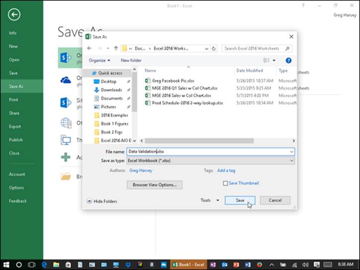
Figure 1-17: Specifying the folder and filename prior to saving the new workbook file.

When you finish making changes in the Save As dialog box, click the Save button or press Enter to have Excel 2016 save your work. When Excel saves your workbook file, the program saves all the information in every worksheet in your workbook (including the last position of the cell cursor) in the designated folder and drive.

You don’t have to fool with the Save As dialog box ever again after initially saving a workbook unless you want to save a copy of the workbook under a new filename and/or in a new folder. If you want to do either of these things, you must choose File  ⇒  Save As or press Alt+FA to choose the Save As command rather than click the Save button on the Quick Access toolbar or press Ctrl+S. Then, select the folder where you want the new version of the file saved if it’s different from the current folder, and you can edit the workbook’s filename if you also want to rename the workbook file.

The Save As dialog box enables you to change the author or add tags to the new workbook file by clicking the Authors or Add a Tag link. You can then use any or all of these pieces of information you add to the file when later searching for the workbook. By default, the Save Thumbnail check box is selected, enabling Excel to display a thumbnail preview of the workbook in the Preview pane of the Open dialog box. (See Book II, Chapter 3 for details.)

Saving workbooks in other commonly used file formats

When you click the Save As Type drop-down button in the Save As dialog box, Excel displays a long laundry list of file formats that you can choose from when saving the workbook file. You can use these file format options to instantly convert your worksheet data into another file format for use with applications other than Excel 2016.

Before saving a new workbook file in a non-Excel file format for use with another type of program (such as Web Page for the Internet, or PDF for the Adobe reader), be sure that you’ve first saved the spreadsheet data in a regular Excel Workbook file. That way, you continue to have ready access to the data in Excel 2016 for the purposes of further editing, printing, and so forth without having to convert the new file back into a native Excel Workbook file format.

The most commonly used file format options include the following:

· Excel Workbook: Saves the workbook in the default Excel 2016 .xlsx file format.

· Excel Macro-Enabled Workbook: Saves the workbook in the default .xlsm file format with all macros (see Book VIII, Chapter 1) it contains enabled.

· Excel Binary Workbook: Saves the workbook in the binary file format optimized that enables faster loading of really large workbooks with tons of data.

· Excel 97-2003 Workbook: Saves the workbook in the .xls file format used by earlier versions of Excel 97 through Excel 2003 — note that an alert dialog box appears if Excel finds any features used in the workbook that aren’t supported in this file format.

· XML Data: Saves the workbook in an XML (Extensible Markup Language) format (using the .xml filename extension) often used to exchange lists of data over the Internet.

· Single File Web Page: Saves the workbook in an MIME HTML (Multipurpose Internet Mail Extension Hypertext Markup Language) with the .mhtm or .mhtml file extension. This special HTML format is used by some web browsers (mainly Internet Explorer) to mimic the worksheets in the original workbook through the use of tabbed pages in the resulting web page.

· Web Page: Saves the workbook in an HTML (Hypertext Markup Language) used to render all the data on all worksheets in the workbook in a single continuous web page with the .htm or .html filename extension.

· Excel Template: Saves the workbook in the .xltx file format as an Excel template file that you can use to generate new workbooks containing the same layout and content as the template.

· Excel Macro-Enabled Template: Saves the workbook in the .xltx template file format with all the macros (see Book VIII, Chapter 1) it contains enabled.

· PDF: Saves the workbook in an Adobe PDF (Portable Document File) format with the .pdf filename extension that can be opened with the free Adobe Reader program.

· XPS Document: Saves the workbook in an XPS (XML Paper Specification) file with the .xps filename extension used by many printers to render the data in a document, including Microsoft Office programs.

· OpenDocument Spreadsheet: Saves the workbook in ODF (OpenDocument Format) with an .ods filename extension that’s used by other Office suites of programs, particularly Sun Microsystems’s StarOffice suite.

Although less frequently needed, don’t forget that the Save As options include a number of text file conversions that you can use when your spreadsheet contains lists of data that you need to make available to programs that can deal with strings of text data. The major difference between the various text file formats is what character they use to separate the data in each worksheet cell. So, the various Text (.txt) formats use tabs, the various comma-separated value (or CSV, .csv) formats use commas, and the various text (.txt) formats use spaces.

Changing the default file location

Whenever you select the Computer button on the Save As screen in the Backstage view to save a new workbook file locally (as opposed to in the cloud on a SharePoint site or your OneDrive), Excel 2016 automatically selects the folder listed in the Default File Location text box on the Save tab of the Excel Options dialog box (File  ⇒  Options  ⇒  Save or Alt+FTS).

If you don’t have a OneDrive or don’t ever save workbook files in the cloud, you can prevent Excel 2016 from asking you to sign into your OneDrive location when saving a new workbook by deselecting the Show Additional Places for Saving, Even If Sign-In May Be Required check box on the Save tab of the Excel Options dialog box. Also, if you prefer selecting the drive and folder into which to save your workbook files directly in the Save As dialog box, you can prevent Excel 2016 from initially displaying the Save As screen by selecting the Don’t Show the Backstage When Opening or Saving Files check box on this same tab of the Excel Options dialog box.

The very generic Documents folder may not be the place on your hard drive where you want all the new workbooks you create automatically saved. To change the default file location to another folder on your computer, follow these steps:

1. Choose File  ⇒  Options  ⇒  Save or press Alt+FTS to open the Save tab of the Excel Options dialog box.

The Default File Location text box displays the directory path to the current default folder.

2. Click the Default File Location text box to select the current directory path.

When you click the Default File Location text box, Excel selects the entire directory path so that if you begin typing, the characters you type replace the entire path. To edit part of the path (such as the Documents folder name after your user name), click the mouse or Touch pointer at that place in the path to set the Insertion point.

3. Edit the existing path or replace it with the path to another existing folder in which you want all future workbooks to automatically be saved.

4. Click OK to close the Excel Options dialog box.

Saving a new workbook in the old file format

Excel 2016 automatically saves each new workbook file in a Microsoft version of the XML-based file format, which carries the filename extension .xlsx. The problem with this XML file format is that it’s not one that versions of Excel prior to Excel 2007 can open. This means that if everybody who needs to work with the workbook you’ve just created hasn’t yet upgraded to Excel 2007 or 2010, you need to save the new workbook in the earlier file format used in versions 97 through 2003 with the old .xls filename extension.

To save a new workbook in the old binary Excel file format for back compatibility, be sure to click the Save as Type drop-down button and then select Excel 97-2003 Workbook from the drop-down list.

Excel automatically displays the Excel Compatibility Checker dialog box whenever you try to save a workbook file containing Excel 2016 features that aren’t supported in earlier versions of the program from Excel 97 through 2003. This dialog box lists each incompatible feature in the workbook and gives you details on what will happen to the feature if you go ahead and save the workbook file in the older file format. To ignore these warnings and go ahead and save your workbook in the 97-2003 binary format, click the Continue button in the Excel Compatibility Checker dialog box.

If you still want to have access to all the features in the Excel 2016 workbook but you still need to create a backwardly compatible version of the workbook file (even if it has less fidelity), first save the workbook in the XML file format with the .xlsx file extension. Then, save a copy in old 97-2003 binary file format with the .xls file extension by opening the Save As dialog box (File  ⇒  Save As or Alt+FA) and then selecting Excel 97-2003 from the Save as Type drop-down list before clicking the Save button.

Keep in mind that filename extensions such as .xlsx and .xls do not appear as part of the filename (even though they are appended) in the File Name text box in the Save As dialog box unless you’ve removed the check mark from the Hide Extensions for Known File Types check box found on the View tab of the Folder Options dialog box (Tools  ⇒  Options) in the Windows Explorer window.

Document Recovery to the Rescue

Excel 2016 offers a document recovery feature that can help you in the event of a computer crash because of a power failure or some sort of operating system freeze or shutdown. The AutoRecover feature saves your workbooks at regular intervals. In the event of a computer crash, Excel displays a Document Recovery Task pane the next time you start Excel after rebooting the computer.

When you first start using Excel 2016, the AutoRecover feature is set to automatically save changes to your workbook (provided that the file has already been saved) every ten minutes. You can shorten or lengthen this interval as you see fit. Choose File  ⇒  Options  ⇒  Save or press Alt+FTS to open the Excel Options dialog box with the Save tab selected. Use the spinner buttons or enter a new automatic save interval into the Save AutoRecover Information Every 10 Minutes text box before clicking OK.

The Document Recovery Task pane shows the available versions of the workbook files that were open at the time of the computer crash. It identifies the original version of the workbook file and when it was saved, along with the recovered version of the file and when it was saved. To open the recovered version of a workbook (to see how much of the work it contains that was unsaved at the time of the crash), position the mouse pointer over the AutoRecover version. Then click its drop-down menu button and click Open on its pop-up menu. After you open the recovered version, you can (if you choose) then save its changes by clicking the Save button on the Quick Access toolbar or by choosing File  ⇒  Save.

You then have these choices:

· To save the recovered version of a workbook without bothering to first open it, place your mouse over the recovered version, click its drop-down button, and choose the Save As option on the pop-up menu.

· To permanently abandon the recovered version (leaving you with only the data in the original version), click the Close button at the bottom of the Document Recovery Task pane. When you click the Close button, an alert dialog box appears, giving you the chance to retain the recovered versions of the file for later viewing.

· To retain the files for later viewing, select the Yes (I Want to View These Files Later) radio button before clicking OK.

· To retain only the original versions of the files shown in the Task pane, select the No (Remove These Files. I Have Saved the Files I Need) radio button instead.

The AutoRecover feature only works on Excel workbooks that have been saved at least one time (as explained in the earlier section “Saving the Data”). In other words, if you build a new workbook and don’t bother to save and rename it prior to experiencing a computer crash, the AutoRecover feature will not bring back any part of it. For this reason, it’s really important that you get into the habit of saving new workbooks with the Save button on the Quick Access toolbar very shortly after beginning to work on a worksheet. Or you can use the trusty keyboard shortcut Ctrl+S.