Microsoft Excel 2016 BIBLE (2016)

Formulas and worksheet functions are essential to manipulating data and obtaining useful information from your Excel workbooks. The chapters in this part present a wide variety of formula examples that use many Excel functions. Two of the chapters are devoted to array formulas. These chapters are intended primarily for advanced users who need to perform calculations that may otherwise be impossible.

IN THIS PART

1. Chapter 10
Introducing Formulas and Functions

2. Chapter 11
Creating Formulas That Manipulate Text

3. Chapter 12
Working with Dates and Times

4. Chapter 13
Creating Formulas That Count and Sum

5. Chapter 14
Creating Formulas That Look Up Values

6. Chapter 15
Creating Formulas for Financial Applications

7. Chapter 16
Miscellaneous Calculations

8. Chapter 17
Introducing Array Formulas

9. Chapter 18
Performing Magic with Array Formulas

IN THIS CHAPTER

1. Understanding formula basics

2. Entering formulas and functions into your worksheets

3. Understanding how to use references in formulas

4. Correcting common formula errors

5. Using advanced naming techniques

6. Getting tips for working with formulas

Formulas are what make a spreadsheet program so useful. If it weren't for formulas, a spreadsheet would simply be a fancy word processing document that has great support for tabular information.

You use formulas in your Excel worksheets to calculate results from the data stored in the worksheet. When data changes, the formulas calculate updated results with no extra effort on your part. This chapter introduces formulas and functions and helps you get up to speed with this important element.

Understanding Formula Basics

A formula consists of special code entered into a cell. It performs a calculation of some type and returns a result that is displayed in the cell. Formulas use a variety of operators and worksheet functions to work with values and text. The values and text used in formulas can be located in other cells, which makes changing data easy and gives worksheets their dynamic nature. For example, you can see multiple scenarios quickly by changing the data in a worksheet and letting your formulas do the work.

A formula always begins with an equal sign and can contain any of these elements:

· Mathematical operators, such as + (for addition) and * (for multiplication)

· Cell references (including named cells and ranges)

· Values or text

· Worksheet functions (such as SUM and AVERAGE)

After you enter a formula, the cell displays the calculated result of the formula. The formula itself appears in the Formula bar when you select the cell, however.

Here are a few examples of formulas:

Note that every formula begins with an equal sign (=). The initial equal sign allows Excel to distinguish a formula from plain text.

Using operators in formulas

Excel formulas support a variety of operators. Operators are symbols that indicate what mathematical (or logical) operation you want the formula to perform. Table 10.1 lists the operators that Excel recognizes. In addition to these, Excel has many built-in functions that enable you to perform additional calculations.

Table 10.1 Operators Used in Formulas

You can, of course, use as many operators as you need to perform the desired calculation.

Here are some examples of formulas that use various operators:

Understanding operator precedence in formulas

When Excel calculates the value of a formula, it uses certain rules to determine the order in which the various parts of the formula are calculated. You need to understand these rules so your formulas produce accurate results.

Table 10.2 lists the Excel operator precedence. This table shows that exponentiation has the highest precedence (performed first) and logical comparisons have the lowest precedence (performed last).

Table 10.2 Operator Precedence in Excel Formulas

You can use parentheses to override Excel's built-in order of precedence. Expressions within parentheses are always evaluated first. For example, the following formula uses parentheses to control the order in which the calculations occur. In this case, cell B3 is subtracted from cell B2, and the result is multiplied by cell B4:

=(B2-B3)*B4

If you enter the formula without the parentheses, Excel computes a different answer. Because multiplication has a higher precedence, cell B3 is multiplied by cell B4. Then this result is subtracted from cell B2, which isn't what was intended.

The formula without parentheses looks like this:

=B2-B3*B4

It's good practice to use parentheses even when they aren't strictly necessary. Doing so helps to clarify what the formula is intended to do. For example, the following formula makes it perfectly clear that B3 should be multiplied by B4 and the result subtracted from cell B2. Without the parentheses, you would need to remember Excel's order of precedence.

=B2-(B3*B4)

You can also nest parentheses within formulas — that is, put them inside other parentheses. If you do so, Excel evaluates the most deeply nested expressions first — and then works its way out. Here's an example of a formula that uses nested parentheses:

=((B2*C2)+(B3*C3)+(B4*C4))*B6

This formula has four sets of parentheses — three sets are nested inside the fourth set. Excel evaluates each nested set of parentheses and then sums the three results. This result is then multiplied by the value in cell B6.

Although the preceding formula uses four sets of parentheses, only the outer set is really necessary. If you understand operator precedence, it should be clear that you can rewrite this formula as follows:

=(B2*C2+B3*C3+B4*C4)*B6

But most would agree that using the extra parentheses makes the calculation much clearer.

Every left parenthesis, of course, must have a matching right parenthesis. If you have many levels of nested parentheses, keeping them straight can sometimes be difficult. If the parentheses don't match, Excel displays a message explaining the problem — and won't let you enter the formula.

Caution

In some cases, if your formula contains mismatched parentheses, Excel may propose a correction to your formula. Figure 10.1 shows an example of a proposed correction. You may be tempted simply to accept Excel's suggestion, but be careful — in many cases, the proposed formula, although syntactically correct, isn't the formula you intended, and it will produce an incorrect result.

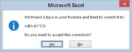
Figure 10.1 Excel sometimes suggests a syntactically correct formula, but not the formula you had in mind.

Tip

When you're editing a formula, Excel lends a hand in helping you match parentheses by displaying matching parentheses in the same color.

Using functions in your formulas

Many formulas you create use worksheet functions. These functions enable you to greatly enhance the power of your formulas and perform calculations that are difficult (or even impossible) if you use only the operators discussed previously. For example, you can use the TAN function to calculate the tangent of an angle. You can't do this complicated calculation by using the mathematical operators alone.

Examples of formulas that use functions

A worksheet function can simplify a formula significantly.

Here's an example. To calculate the average of the values in ten cells (A1:A10) without using a function, you'd have to construct a formula like this:

=(A1+A2+A3+A4+A5+A6+A7+A8+A9+A10)/10

Not very pretty, is it? Even worse, you would need to edit this formula if you added another cell to the range. Fortunately, you can replace this formula with a much simpler one that uses one of Excel's built-in worksheet functions, AVERAGE:

=AVERAGE(A1:A10)

The following formula demonstrates how using a function can enable you to perform calculations that are not otherwise possible. Say you need to determine the largest value in a range. A formula can't tell you the answer without using a function. Here's a formula that uses the MAX function to return the largest value in the range A1:D100:

=MAX(A1:D100)

Functions also can sometimes eliminate manual editing. Assume that you have a worksheet that contains 1,000 names in cells A1:A1000 and the names appear in all-capital letters. Your boss sees the listing and informs you that the names will be mail-merged with a form letter. Use of all-uppercase letters is not acceptable; for example, JOHN F. SMITH must now appear as John F. Smith. You could spend the next several hours re-entering the list (ugh), or you could use a formula, such as the following, which uses the PROPER function to convert the text in cell A1 to the proper case:

=PROPER(A1)

Enter this formula once in cell B1 and then copy it down to the next 999 rows. Then select B1:B1000 and choose Home Clipboard Copy to copy the range. Next, with B1:B1000 still selected, choose Home Clipboard Paste Values (V) to convert the formulas to values. Delete the original column, and you've just accomplished several hours of work in less than a minute.

Tip

You can also use Excel's Flash Fill feature to make this type of transformation, without formulas. See Chapter 32, “Importing and Cleaning Data,” for more about Flash Fill.

One last example should convince you of the power of functions. Suppose you have a worksheet that calculates sales commissions. If the salesperson sold more than $100,000 of product, the commission rate is 7.5 percent; otherwise, the commission rate is 5.0 percent. Without using a function, you would have to create two different formulas and make sure that you use the correct formula for each sales amount. A better solution is to write a formula that uses the IF function to ensure that you calculate the correct commission, regardless of sales amount:

=IF(A1<100000,A1*5%,A1*7.5%)

This formula performs some simple decision making. The formula checks the value of cell A1, which contains the sales amount. If this value is less than 100,000, the formula returns cell A1 multiplied by 5 percent. Otherwise, it returns what's in cell A1 multiplied by 7.5 percent. This example uses three arguments, separated by commas. I discuss this in the next section, “Function arguments.”

Function arguments

In the preceding examples, you may have noticed that all the functions used parentheses. The information inside the parentheses is the list of arguments.

Functions vary in the way they use arguments. Depending on what it has to do, a function may use

· No arguments

· One argument

· A fixed number of arguments

· An indeterminate number of arguments

· Optional arguments

An example of a function that doesn't use an argument is the NOW function, which returns the current date and time. Even if a function doesn't use an argument, you must still provide a set of empty parentheses, like this:

=NOW()

If a function uses more than one argument, separate each argument with a comma. The examples at the beginning of the chapter used cell references for arguments. Excel is quite flexible when it comes to function arguments, however. An argument can consist of a cell reference, literal values, literal text strings, expressions, and even other functions. Here are some examples of functions that use various types of arguments:

· Cell reference: =SUM(A1:A24)

· Literal value: =SQRT(121)

· Literal text string: =PROPER("john f. smith")

· Expression: =SQRT(183+12)

· Other functions: =SQRT(SUM(A1:A24))

Note

A comma is the list separator character for the U.S. version of Excel. Some other language versions may use a semicolon. The list separator is a Windows setting that can be adjusted in the Windows Control Panel (the Regional and Language Options dialog box).

More about functions

All told, Excel includes more than 450 built-in functions. And if that's not enough, you can download or purchase additional specialized functions from third-party suppliers — and even create your own custom functions (by using VBA) if you're so inclined.

Some users feel a bit overwhelmed by the sheer number of functions, but you'll probably find that you use only a dozen or so on a regular basis. And as you'll see, the Excel Insert Function dialog box (described later in this chapter) makes it easy to locate and insert a function, even if it's not one that you use frequently.

You'll find many examples of Excel's built-in functions in Part II, “Working with Formulas and Function.” Appendix A, “Worksheet Function Reference,” contains a complete listing of Excel's worksheet functions, with a brief description of each. Chapter 40, “Creating Custom Worksheet Functions,” covers the basics of creating custom functions with VBA.

Entering Formulas into Your Worksheets

Every formula must begin with an equal sign to inform Excel that the cell contains a formula rather than text. Excel provides two ways to enter a formula into a cell: manually or by pointing to cell references. The following sections discuss each method in detail.

Excel provides additional assistance when you create formulas by displaying a drop-down list that contains function names and range names. The items displayed in the list are determined by what you've already typed. For example, if you're entering a formula and then type the letters SU, you'll see the drop-down list shown in Figure 10.2. If you type an additional letter, the list is shortened to show only the matching functions. To have Excel autocomplete an entry in that list, use the navigation keys to highlight the entry, and then press Tab. Notice that highlighting a function in the list also displays a brief description of the function. See the next sidebar, “Using Formula AutoComplete,” for an example of how this feature works.

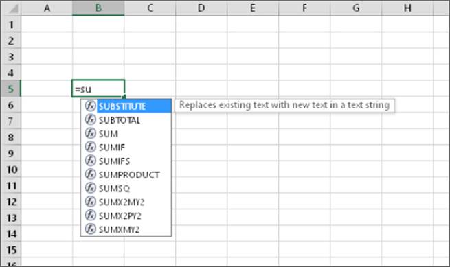
Figure 10.2 Excel displays a drop-down list when you enter a formula.

Using Formula AutoComplete

The Formula AutoComplete feature makes entering formulas easier than ever. Here's a quick walk-through that demonstrates how it works. The goal is to create a formula that uses the AGGREGATE function to calculate the average value in a range that I named TestScores. The AVERAGE function will not work in this situation because the range contains an error value.

1. Select the cell that will hold the formula, and type an equal sign (=) to signal the start of a formula.

2. Type the letter A. You get a list of functions and names that begin with A (see the figure). This feature is not case sensitive, so you can use either uppercase or lowercase characters.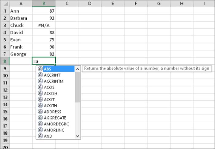

3. Scroll through the list, or type another letter to narrow down the choices.

4. WhenAGGREGATEis highlighted, press Tab to select it. Excel adds the opening parenthesis and displays another list that contains options for the first argument for AGGREGATE, as shown in the figure.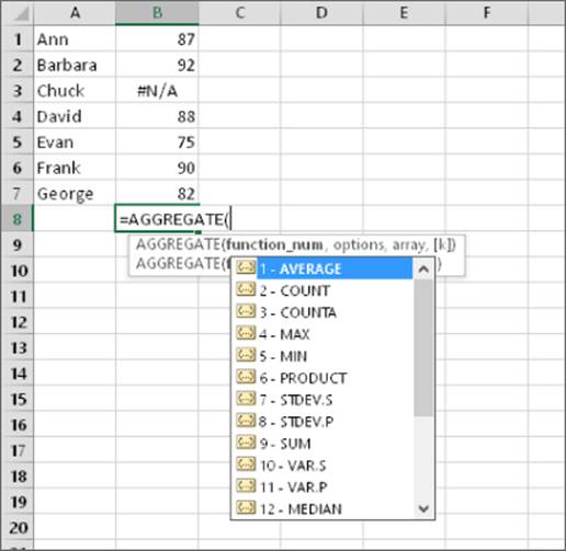

5. Select1 - AVERAGEand then press Tab. Excel inserts 1, which is the code for calculating the average.

6. Type a comma to separate the next argument.

7. When Excel displays a list of items for theAGGREGATEfunction's second argument, select2 - Ignore Error Valuesand then press Tab.

8. Type a comma to separate the third argument (the range of test scores).

9. Type a T to get a list of functions and names that begin with T; you're looking forTestScores, so narrow it down a bit by typing the second character, E.

10.HighlightTestScores, and then press Tab.

11.Type a closing parenthesis and then press Enter.

The completed formula follows:

=AGGREGATE(1,2,TestScores)

Formula AutoComplete includes the following items (and each type is identified by an icon):

· Excel built-in functions.

· User-defined functions (functions defined by the user through VBA or other methods).

· Defined names (cells or range named using the Formulas Defined Names Define Name command).

· Enumerated arguments that use a value to represent an option. (Only a few functions use such arguments, and AGGREGATE is one of them.)

· Table structure references (used to identify portions of a table).

Entering formulas manually

Entering a formula manually involves, well, entering a formula manually. In a selected cell, you type an equal sign (=) followed by the formula. As you type, the characters appear in the cell and in the Formula bar. You can, of course, use all the normal editing keys when entering a formula.

Entering formulas by pointing

Even though you can enter formulas by typing in the entire formula, Excel provides another method of entering formulas that is generally easier, faster, and less error prone. This method still involves some manual typing, but you can simply point to the cell references instead of typing their values manually. For example, to enter the formula =A1+A2 into cell A3, follow these steps:

1. Move the cell pointer to cell A3.

2. Type an equal sign (=) to begin the formula. Notice that Excel displays Enter in the status bar (lower left of your screen).

3. Press the up arrow twice. As you press this key, Excel displays a dashed border around cell A1, and the cell reference appears in cell A3 and in the Formula bar. In addition, Excel displays Point in the status bar.

4. Type a plus sign (+). A solid color border replaces the dashed border of A1, and Enter reappears in the status bar.

5. Press the up arrow again. The dashed border encompasses cell A2 and adds that cell address to the formula.

6. Press Enter to end the formula.

Tip

When creating a formula by pointing, you can also point to the data cells by using your mouse.

Pasting range names into formulas

If your formula uses named cells or ranges, you can either type the name in place of the address or choose the name from a list and have Excel insert the name for you automatically. Two ways to insert a name into a formula are available:

· Select the name from the drop-down list. To use this method, you must know at least the first character of the name. When you're entering the formula, type the first character and then select the name from the drop-down list.

· Press F3. The Paste Name dialog box appears. Select the name from the list and then click OK (or just double-click the name). Excel enters the name into your formula. If no names are defined, pressing F3 has no effect.

Figure 10.3 shows an example. The worksheet contains two defined names: Expenses and Sales. The Paste Name dialog box is being used to insert a name (Sales) into the formula being entered in cell B9.

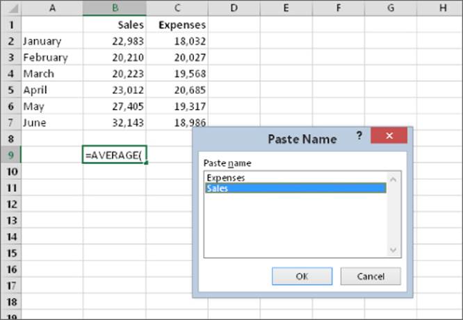
Figure 10.3 Use the Paste Name dialog box to quickly enter a defined name into a formula.

See Chapter 4, “Working with Cells and Ranges,” for information about creating names for cells and ranges.

Inserting functions into formulas

The easiest way to enter a function into a formula is to use Formula AutoComplete (the drop-down list that Excel displays while you type a formula). To use this method, however, you must know at least the first character of the function's name.

Another way to insert a function is to use tools in the Function Library group on the Formulas tab on the Ribbon (see Figure 10.4). This method is especially useful if you can't remember which function you need. When entering a formula, click the function category (Financial, Logical, Text, and so on) to get a list of the functions in that category. Click the function you want, and Excel displays its Function Arguments dialog box. This is where you enter the function's arguments. In addition, you can click the Help on This Function link to learn more about the selected function.

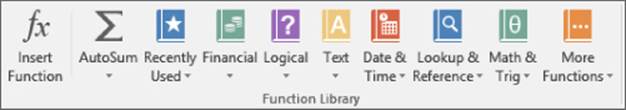
Figure 10.4 You can insert a function by selecting it from one of the function categories.

Yet another way to insert a function into a formula is to use the Insert Function dialog box (see Figure 10.5). You can access this dialog box in several ways:

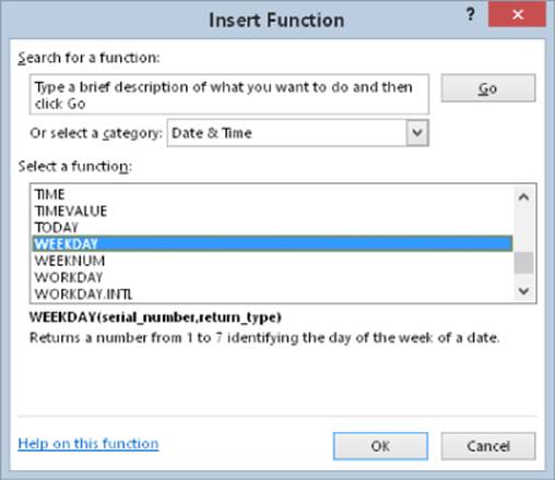
Figure 10.5 The Insert Function dialog box.

· Choose Formulas Function Library Insert Function.

· Use the Insert Function command, which appears at the bottom of each drop-down list in the Formulas Function Library group.

· Click the Insert Function icon, which is directly to the left of the Formula bar. This button displays fx.

· Press Shift+F3.

The Insert Function dialog box shows a drop-down list of function categories. Select a category, and the functions in that category are displayed in the list box. To access a function that you recently used, select Most Recently Used from the drop-down list.

If you're not sure which function you need, you can search for the appropriate function by using the Search for a Function field at the top of the dialog box.

1. Enter your search terms and click Go. You get a list of relevant functions. When you select a function from the Select a Function list, Excel displays the function (and its argument names) in the dialog box along with a brief description of what the function does.

2. When you locate the function you want to use, highlight it and click OK. Excel then displays its Function Arguments dialog box, as shown in Figure 10.6.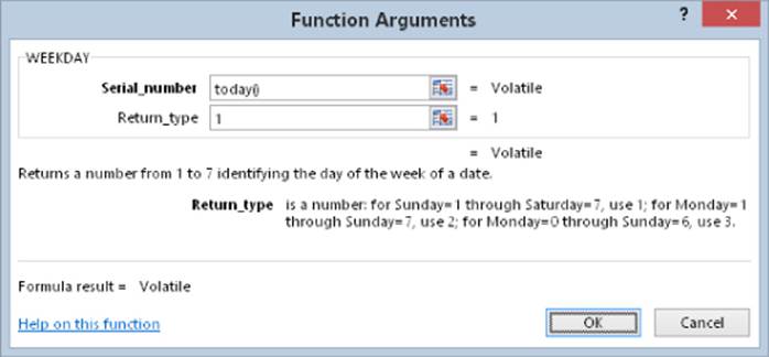

Figure 10.6 The Function Arguments dialog box.

3. Specify the arguments for the function. The Function Arguments dialog box will vary, depending on the function you're inserting, and it will show one text box for each of the function's arguments. To use a cell or range reference as an argument, you can enter the address manually or click inside the argument box and then select (that is, point to) the cell or range in the sheet.

4. After you specify all the function arguments, click OK.

Tip

Yet another way to insert a function while you're entering a formula is to use the Function List to the left of the Formula bar. When you're entering or editing a formula, the space typically occupied by the Name box displays a list of the functions you've used most recently (if any). After you select a function from this list, Excel displays the Function Arguments dialog box.

Function entry tips

Here are some additional tips to keep in mind when you use the Insert Function dialog box to enter functions:

· You can use the Insert Function dialog box to insert a function into an existing formula. Just edit the formula and move the insertion point to the location at which you want to insert the function. Then open the Insert Function dialog box (using any of the methods described earlier) and select the function.

· You can also use the Function Arguments dialog box to modify the arguments for a function in an existing formula. Click the function in the Formula bar and then click the Insert Function button (the fx button, to the left of the Formula bar).

· If you change your mind about entering a function, click the Cancel button.

· The number of boxes you see in the Function Arguments dialog box depends on the number of arguments used in the function you selected. If a function uses no arguments, you won't see any boxes. If the function uses a variable number of arguments (such as the AVERAGE function), Excel adds a new box every time you enter an optional argument.

· As you provide arguments in the Function Arguments dialog box, the value of each argument is displayed to the right of each box.

· A few functions, such as INDEX, have more than one form. If you choose such a function, Excel displays another dialog box that lets you choose which form you want to use.

· As you become familiar with the functions, you can bypass the Insert Function dialog box and type the function name directly. Excel prompts you with argument names as you enter the function.

Editing Formulas

After you enter a formula, you can (of course) edit it. You may need to edit a formula if you make some changes to your worksheet and then have to adjust the formula to accommodate the changes. Or the formula may return an error value, in which case you need to edit the formula to correct the error.

Notice that Excel color-codes the range addresses and ranges when you're entering or editing a formula. This helps you quickly spot the cells that are used in a formula.

Here are some of the ways to get into cell edit mode:

· Double-click the cell, which enables you to edit the cell contents directly in the cell.

· Press F2, which enables you to edit the cell contents directly in the cell.

· Select the cell that you want to edit, and then click in the Formula bar. This enables you to edit the cell contents in the Formula bar.

· If the cell contains a formula that returns an error, Excel will display a small triangle in the upper-left corner of the cell. Activate the cell, and you'll see a Smart Tag. Click the Smart Tag, and you can choose one of the options for correcting the error. (The options will vary according to the type of error in the cell.)

Tip

You can control whether Excel displays these formula-error-checking Smart Tags in the Formulas section of the Excel Options dialog box. To display this dialog box, choose File Options. If you remove the check mark from Enable Background Error Checking, Excel no longer displays these Smart Tags.

While you're editing a formula, you can select multiple characters either by dragging the mouse cursor over them or by pressing Shift while you use the navigation keys.

Tip

If you have a formula that you can't seem to edit correctly, you can convert the formula to text and tackle it again later. To convert a formula to text, just remove the initial equal sign (=). When you're ready to try again, type the initial equal sign to convert the cell contents back to a formula.

Using Cell References in Formulas

Most formulas you create include references to cells or ranges. These references enable your formulas to work dynamically with the data contained in those cells or ranges. For example, if your formula refers to cell A1 and you change the value contained in A1, the formula result changes to reflect the new value. If you didn't use references in your formulas, you would need to edit the formulas themselves to change the values used in the formulas.

Using relative, absolute, and mixed references

When you use a cell (or range) reference in a formula, you can use three types of references:

· Relative: The row and column references can change when you copy the formula to another cell because the references are actually offsets from the current row and column. By default, Excel creates relative cell references in formulas.

· Absolute: The row and column references don't change when you copy the formula because the reference is to an actual cell address. An absolute reference uses two dollar signs in its address: one for the column letter and one for the row number (for example, $A$5).

· Mixed: Either the row or the column reference is relative, and the other is absolute. Only one of the address parts is absolute (for example, $A4 or A$4).

The type of cell reference is important only if you plan to copy the formula to other cells. The following examples illustrate this point.

Figure 10.7 shows a simple worksheet. The formula in cell D2, which multiplies the quantity by the price, is

=B2*C2

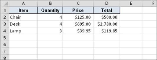
Figure 10.7 Copying a formula that contains relative references.

This formula uses relative cell references. Therefore, when the formula is copied to the cells below it, the references adjust in a relative manner. For example, the formula in cell D3 is

=B3*C3

But what if the cell references in D2 contained absolute references, like this?

=$B$2*$C$2

In this case, copying the formula to the cells below would produce incorrect results. The formula in cell D3 would be the same as the formula in cell D2.

Now I'll extend the example to calculate sales tax, which is stored in cell B7 (see Figure 10.8). In this situation, the formula in cell D2 is

=(B2*C2)*$B$7

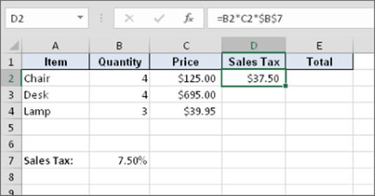
Figure 10.8 Formula references to the sales tax cell should be absolute.

The quantity is multiplied by the price, and the result is multiplied by the sales tax rate stored in cell B7. Notice that the reference to B7 is an absolute reference. When the formula in D2 is copied to the cells below it, cell D3 will contain this formula:

=(B3*C3)*$B$7

Here, the references to cells B2 and C2 were adjusted, but the reference to cell B7 was not — which is exactly what I want because the address of the cell that contains the sales tax never changes.

Figure 10.9 demonstrates the use of mixed references. The formulas in the C3:F7 range calculate the area for various lengths and widths. Here's the formula in cell C3:

=$B3*C$2

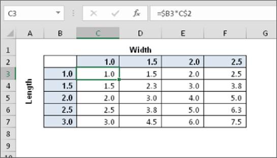
Figure 10.9 Using mixed cell references.

Notice that both cell references are mixed. The reference to cell B3 uses an absolute reference for the column ($B), and the reference to cell C2 uses an absolute reference for the row ($2). As a result, this formula can be copied down and across, and the calculations will be correct. For example, the formula in cell F7 is

=$B7*F$2

If C3 used either absolute or relative references, copying the formula would produce incorrect results.

A workbook that demonstrates the various types of references is available on this book's website at www.wiley.com/go/excel2016bible. The file is named cell references.xlsx.

Note

When you cut and paste a formula (move it to another location), the cell references in the formula aren't adjusted. Again, this is usually what you want to happen. When you move a formula, you generally want it to continue to refer to the original cells.

Changing the types of your references

You can enter nonrelative references (that is, absolute or mixed) manually by inserting dollar signs in the appropriate positions of the cell address. Or you can use a handy shortcut: the F4 key. When you've entered a cell reference (by typing it or by pointing), you can press F4 repeatedly to have Excel cycle through all four reference types.

For example, if you enter =A1 to start a formula, pressing F4 converts the cell reference to =$A$1. Pressing F4 again converts it to =A$1. Pressing it again displays =$A1. Pressing it one more time returns to the original =A1. Keep pressing F4 until Excel displays the type of reference that you want.

Note

When you name a cell or range, Excel (by default) uses an absolute reference for the name. For example, if you give the name SalesForecast to B1:B12, the Refers To box in the New Name dialog box lists the reference as $B$1:$B$12. This is almost always what you want. If you copy a cell that has a named reference in its formula, the copied formula contains a reference to the original name.

Referencing cells outside the worksheet

Formulas can also refer to cells in other worksheets — and the worksheets don't even have to be in the same workbook. Excel uses a special type of notation to handle these types of references.

Referencing cells in other worksheets

To use a reference to a cell in another worksheet in the same workbook, use this format:

SheetName!CellAddress

In other words, precede the cell address with the worksheet name, followed by an exclamation point. Here's an example of a formula that uses a cell on the Sheet2 worksheet:

=A1*Sheet2!A1

This formula multiplies the value in cell A1 on the current worksheet by the value in cell A1 on Sheet2.

Tip

If the worksheet name in the reference includes one or more spaces, you must enclose it in single quotation marks. (Excel does that automatically if you use the point-and-click method when creating the formula.) For example, here's a formula that refers to a cell on a sheet named All Depts:

=A1*'All Depts'!A1

Referencing cells in other workbooks

To refer to a cell in a different workbook, use this format:

=[WorkbookName]SheetName!CellAddress

In this case, the workbook name (in square brackets), the worksheet name, and an exclamation point precede the cell address. The following is an example of a formula that uses a cell reference in the Sheet1 worksheet in a workbook named Budget:

=[Budget.xlsx]Sheet1!A1

If the workbook name in the reference includes one or more spaces, you must enclose it (and the sheet name and square brackets) in single quotation marks. For example, here's a formula that refers to a cell on Sheet1 in a workbook named Budget For 2016:

=A1*'[Budget For 2016.xlsx]Sheet1'!A1

When a formula refers to cells in a different workbook, the other workbook doesn't have to be open. If the workbook is closed, however, you must add the complete path to the reference so that Excel can find it. Here's an example:

=A1*'C:\My Documents\[Budget For 2016.xlsx]Sheet1'!A1

A linked file can also reside on another system that's accessible on your corporate network. The following formula refers to a cell in a workbook in the files directory of a computer named DataServer:

='\\DataServer\files\[budget.xlsx]Sheet1'!$D$7

See Chapter 28, “Linking and Consolidating Worksheets,” for more information about linking workbooks.

Tip

To create formulas that refer to cells in a different worksheet, point to the cells rather instead of entering their references manually. Excel takes care of the details regarding the workbook and worksheet references. The workbook you're referencing in your formula must be open if you're going to use the pointing method.

Note

If you point to a different worksheet or workbook when creating a formula, you'll notice that Excel always inserts absolute cell references. Therefore, if you plan to copy the formula to other cells, make sure that you change the cell references to relative before you copy.

Using Formulas in Tables

A table is a specially designated range of cells, set up with column headers. In this section, I describe how formulas work with tables.

See Chapter 5, “Introducing Tables,” for an introduction to the Excel table features.

Summarizing data in a table

Figure 10.10 shows a simple table with three columns. I entered the data and then converted the range to a table by choosing Insert Tables Table. Note that I didn't define any names, but the table is named Table1 by default.

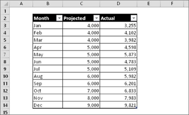
Figure 10.10 A simple table with three columns of information.

This workbook is available on this book's website at www.wiley.com/go/excel2016bible. It is named table formulas.xlsx.

If you'd like to calculate the total projected and total actual sales, you don't even need to write a formula. Simply click a button to add a row of summary formulas to the table:

1. Activate any cell in the table.

2. Place a check mark next to Table Tools Design Table Style Options Total Row. Excel adds a total row to the table and displays the sum of each numeric column.

3. To change the type of summary formula, activate a cell in the total row and use the drop-down list to change the type of summary formula to use (see Figure 10.11). For example, to calculate the average of the Actual column, selectAVERAGE from the drop-down list in cell D15. Excel creates this formula:

=SUBTOTAL(101,[Actual])

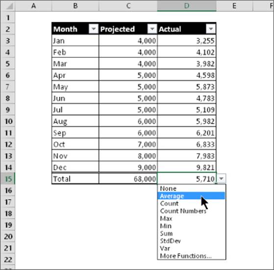
Figure 10.11 A drop-down list enables you to select a summary formula for a table column.

For the SUBTOTAL function, 101 is an enumerated argument that represents AVERAGE. The second argument for the SUBTOTAL function is the column name, in square brackets. Using the column name within brackets creates “structured” references within a table. (I discuss this further in the upcoming section “Referencing data in a table.”)

Note

You can toggle the total row display via Table Tools Design Table Style Options Total Row. If you turn it off, the summary options you selected will be displayed again when you turn it back on.

Using formulas within a table

In many cases, you'll want to use formulas within a table to perform calculations that use other columns in the table. For example, in the table shown in Figure 10.11, you may want a column that shows the difference between the Actual and Projected amounts. To add this formula, follow these steps:

1. Activate cell E2 and type Difference for the column header. Excel automatically expands the table for you to include the new column.

2. Move to cell E3 and type an equal sign to signify the beginning of a formula.

3. Press the left arrow key. Excel displays [@Actual], which is the column heading, in the Formula bar.

4. Type a minus sign and then press the left arrow key twice. Excel displays [@Projected] in your formula.

5. Press Enter to end the formula. Excel copies the formula to all rows in the table.

Figure 10.12 shows the table with the new column.

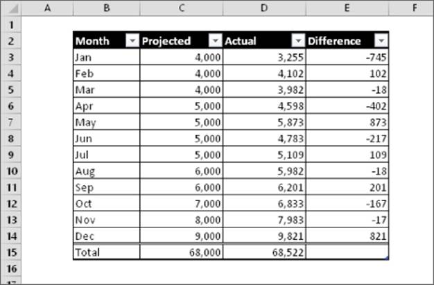
Figure 10.12 The Difference column contains a formula.

Examine the table, and you find this formula for all cells in the Difference column:

=[@Actual]-[@Projected]

Although the formula was entered into the first row of the table, that's not necessary. Any time a formula is entered into an empty table column, it will automatically fill all the cells in that column. And if you need to edit the formula, Excel will automatically copy the edited formula to the other cells in the column.

Note

The at symbol (@) that precedes the column header represents “this row.” So [@Actual] means “the value in the Actual column in this row.”

These steps use the pointing technique to create the formula. Alternatively, you could have entered the formula manually using standard cell references rather than column headers. For example, you could have entered the following formula in cell E3:

=D3-C3

If you type the cell references, Excel will still copy the formula to the other cells automatically.

One thing should be clear, however, about formulas that use the column headers instead of cell references: they're much easier to understand.

Tip

To override the automatic column formulas, access the Proofing tab of the Excel Options dialog box. Click AutoCorrect Options and then select the AutoFormat As You Type tab in the AutoCorrect dialog box. Remove the checkmark from Fill Formulas in Tables to Create Calculated Columns.

Referencing data in a table

Excel offers some other ways to refer to data that's contained in a table by using the table name and column headers.

Note

Remember that you don't need to create names for tables and columns. The data in the table itself has a range name, which is created automatically when you create the table (for example, Table1), and you can refer to data within the table by using the column headers — which are not range names.

You can, of course, use standard cell references to refer to data in a table, but using the table name and column headers has a distinct advantage: the names adjust automatically if the table size changes by adding or deleting rows. In addition, formulas that use table names and column headers will adjust automatically if you change the name of the table or give a new name to a column.

Refer to the table shown in Figure 10.11. This table is named Table1. To calculate the sum of all the data in the table, enter this formula into a cell outside the table:

=SUM(Table1)

This formula will return the sum of all the data (excluding calculated total row values, if any), even if rows or columns are added or deleted. And if you change the name of Table1, Excel will adjust formulas that refer to that table automatically. For example, if you renamed Table1 to AnnualData (by using the Name Manager or by choosing Table Tools Design Properties Table Name), the preceding formula would change to

=SUM(AnnualData)

Most of the time, a formula will refer to a specific column in the table. The following formula returns the sum of the data in the Actual column:

=SUM(Table1[Actual])

Notice that the column name is enclosed in square brackets. Again, the formula adjusts automatically if you change the text in the column heading.

Even better, Excel provides some helpful assistance when you create a formula that refers to data within a table. Figure 10.13 shows the formula AutoComplete helping to create a formula by showing a list of the elements in the table. Notice that, in addition to the column headers in the table, Excel lists other table elements that you can reference: #All, #Data, #Headers, #Totals, and @ - This Row.

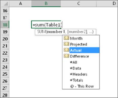
Figure 10.13 The formula AutoComplete feature is useful when creating a formula that refers to data in a table.

Correcting Common Formula Errors

Sometimes when you enter a formula, Excel displays a value that begins with a hash mark (#). This is a signal that the formula is returning an error value. You have to correct the formula (or correct a cell that the formula references) to get rid of the error display.

Tip

If the entire cell is filled with hash-mark characters, the column isn't wide enough to display the value. You can either widen the column or change the number format of the cell.

In some cases, Excel won't even let you enter an erroneous formula. For example, the following formula is missing the closing parenthesis:

=A1*(B1+C2

If you attempt to enter this formula, Excel informs you that you have unmatched parentheses, and it proposes a correction. Often, the proposed correction is accurate, but you can't count on it.

Table 10.3 lists the types of error values that may appear in a cell that has a formula. Formulas may return an error value if a cell to which they refer has an error value. This is known as the ripple effect — a single error value can make its way into lots of other cells that contain formulas that depend on that one cell.

Table 10.3 Excel Error Values

Handling circular references

When you're entering formulas, you may occasionally see a warning message like the one shown in Figure 10.14, indicating that the formula you just entered will result in a circular reference. A circular reference occurs when a formula refers to its own cell — either directly or indirectly. For example, you create a circular reference if you enter =A1+A2+A3 into cell A3 because the formula in cell A3 refers to cell A3. Every time the formula in A3 is calculated, it must be calculated again because A3 has changed. The calculation could go on forever.

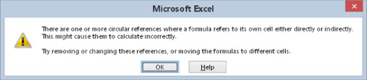
Figure 10.14 If you see this warning, you know that the formula you entered will result in a circular reference.

When you get the circular reference message after entering a formula, Excel gives you two options:

· Click OK to enter the formula as is.

· Click Help to see a Help screen about circular references.

Regardless of which option you choose, Excel displays a message in the left side of the status bar to remind you that a circular reference exists.

Caution

Excel won't tell you about a circular reference if the Enable Iterative Calculation setting is in effect. You can check this setting in the Formulas section of the Excel Options dialog box. If Enable Iterative Calculation is turned on, Excel performs the circular calculation exactly the number of times specified in the Maximum Iterations field (or until the value changes by less than 0.001 or whatever value is in the Maximum Change field). In a few situations, you may use a circular reference intentionally. In these cases, the Enable Iterative Calculation setting must be on. However, it's best to keep this setting turned off so that you're warned of circular references. Usually, a circular reference indicates an error that you must correct.

Often, a circular reference is quite obvious and easy to identify and correct. But when a circular reference is indirect (as when a formula refers to another formula that refers to yet another formula that refers to the original formula), it may require a bit of detective work to get to the problem.

Specifying when formulas are calculated

You've probably noticed that Excel calculates the formulas in your worksheet immediately. If you change any cells that the formula uses, Excel displays the formula's new result with no effort on your part. All this happens when Excel's Calculation mode is set to Automatic. In Automatic Calculation mode (which is the default mode), Excel follows these rules when it calculates your worksheet:

· When you make a change — enter or edit data or formulas, for example — Excel calculates immediately those formulas that depend on new or edited data.

· If Excel is in the middle of a lengthy calculation, it temporarily suspends the calculation when you need to perform other worksheet tasks; it resumes calculating when you're finished with your other worksheet tasks.

· Formulas are evaluated in a natural sequence. In other words, if a formula in cell D12 depends on the result of a formula in cell D24, Excel calculates cell D24 before calculating cell D12.

Sometimes, however, you may want to control when Excel calculates formulas. For example, if you create a worksheet with thousands of complex formulas, you may find that processing can slow to a snail's pace while Excel does its thing. In such a case, set Excel's calculation mode to Manual — which you can do by choosing Formulas Calculation Calculation Options Manual (see Figure 10.15).

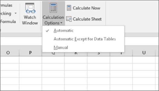
Figure 10.15 You can control when Excel calculates formulas.

Tip

If your worksheet uses any large data tables, you may want to select the Automatic Except for Data Tables option. Large data tables calculate notoriously slowly. A data table is not the same as a table created by choosing Insert Tables Table.

See Chapter 35, “Performing Spreadsheet What-If Analysis,” for more on data tables.

When you're working in Manual Calculation mode, Excel displays Calculate in the status bar when you have any uncalculated formulas. You can use the following shortcut keys to recalculate the formulas:

· F9: Calculates the formulas in all open workbooks.

· Shift+F9: Calculates only the formulas in the active worksheet. Other worksheets in the same workbook aren't calculated.

· Ctrl+Alt+F9: Forces a complete recalculation of all formulas.

· Ctrl+Alt+Shift+F9: Rebuilds the calculation dependency tree and performs a complete recalculation.

Note

Excel's Calculation mode isn't specific to a particular worksheet. When you change the Calculation mode, it affects all open workbooks, not just the active workbook.

Using Advanced Naming Techniques

Using range names can make your formulas easier to understand and modify and even help prevent errors. Dealing with a meaningful name such as AnnualSales is much easier than dealing with a range reference, such as AB12:AB68.

See Chapter 4, “Working with Cells and Ranges,” for basic information regarding working with names.

Excel offers a number of advanced techniques that make using names even more useful. I discuss these techniques in the sections that follow. This information is for those who are interested in exploring some of the aspects of Excel that most users don't even know about.

Using names for constants

Many Excel users don't realize that you can give a name to an item that doesn't appear in a cell. For example, if formulas in your worksheet use a sales tax rate, you would probably insert the tax rate value into a cell and use this cell reference in your formulas. To make things easier, you would probably also name this cell something similar to SalesTax.

Here's how to provide a name for a value that doesn't appear in a cell:

1. Choose Formulas Defined Names Define Name. The New Name dialog box appears.

2. Enter the name (in this case, SalesTax) into the Name field.

3. Select a scope in which the name will be valid (either the entire workbook or a specific worksheet).

4. Click the Refers To text box, delete its contents, and replace the old contents with a value (such as .075).

5. (Optional) Use the Comment box to provide a comment about the name.

6. Click OK to close the New Name dialog box and create the name.

You just created a name that refers to a constant rather than a cell or range. Now if you type =SalesTax into a cell that's within the scope of the name, this simple formula returns 0.075 — the constant that you defined. You can also use this constant in a formula, such as =A1*SalesTax.

Tip

A constant also can be text. For example, you can define a constant for your company's name.

Note

Named constants don't appear in the Name box or in the Go To dialog box. This makes sense because these constants don't reside anywhere tangible. They do appear in the drop-down list that's displayed when you enter a formula — which is handy because you use these names in formulas.

Using names for formulas

In addition to creating named constants, you can create named formulas. Like a named constant, a named formula doesn't reside in a cell.

You create named formulas the same way you create named constants — by using the New Name dialog box. For example, you might create a named formula that calculates the monthly interest rate from an annual rate; Figure 10.16 shows an example. In this case, the name MonthlyRate refers to the following formula:

=Sheet3!$B$1/12

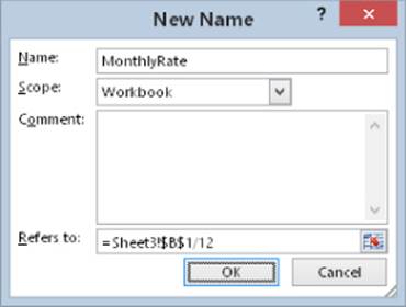
Figure 10.16 Excel allows you to name a formula that doesn't exist in a worksheet cell.

When you use the name MonthlyRate in a formula, it uses the value in B1 divided by 12. Notice that the cell reference is an absolute reference.

Naming formulas gets more interesting when you use relative references rather than absolute references. When you use the pointing technique to create a formula in the Refers To field of the New Name dialog box, Excel always uses absolute cell references — which is unlike its behavior when you create a formula in a cell.

For example, activate cell B1 on Sheet1 and create the name Cubed for the following formula:

=Sheet1!A1^3

In this example, the relative reference points to the cell to the left of the cell in which the name is used. Therefore, make certain that cell B1 is the active cell before you open the New Name dialog box; this is important. The formula contains a relative reference. When you use this named formula in a worksheet, the cell reference is always relative to the cell that contains the formula. For example, if you enter =Cubed into cell D12, cell D12 displays the contents of cell C12 raised to the third power. (C12 is the cell directly to the left of cell D12.)

Using range intersections

This section describes a concept known as range intersections (individual cells that two ranges have in common). Excel uses an intersection operator — a space character — to determine the overlapping references in two ranges. Figure 10.17 shows a simple example.

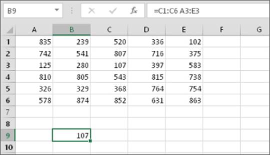
Figure 10.17 You can use a range intersection formula to determine values.

The formula in cell B9 is

=C1:C6 A3:E3

This formula returns 107, the value in cell C3 — that is, the value at the intersection of the two ranges.

The intersection operator is one of three reference operators used with ranges. Table 10.4 lists these operators.

Table 10.4 Reference Operators for Ranges

The real value of knowing about range intersections is apparent when you use names. Examine Figure 10.18, which shows a table of values. I selected the entire table and then chose Formulas Defined Names Create from Selection to create names automatically by using the top row and the left column.

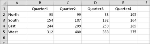
Figure 10.18 With names, using a range intersection formula to determine values is even more helpful.

Excel created the following eight names:

With these names defined, you can create formulas that are easy to read and use. For example, to calculate the total for Quarter 4, just use this formula:

=SUM(Quarter4)

To refer to a single cell, use the intersection operator. Move to any blank cell and enter the following formula:

=Quarter1 West

This formula returns the value for the first quarter for the West region. In other words, it returns the value that exists where the Quarter1 range intersects with the West range. Naming ranges in this manner can help you create very readable formulas.

Applying names to existing references

When you create a name for a cell or a range, Excel doesn't automatically use the name in place of existing references in your formulas. For example, suppose you have the following formula in cell F10:

=A1–A2

If you later define a name Income for A1 and Expenses for A2, Excel won't automatically change your formula to =Income–Expenses. Replacing cell or range references with their corresponding names is fairly easy, however.

To apply names to cell references in formulas after the fact, start by selecting the range that you want to modify. Then choose Formulas Defined Names Define Name Apply Names. The Apply Names dialog box (shown in Figure 10.19) appears. Select the names that you want to apply by clicking them, and then click OK. Excel replaces the range references with the names in the selected cells.

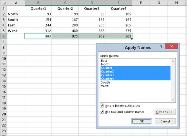
Figure 10.19 Use the Apply Names dialog box to replace cell or range references with defined names.

Working with Formulas

In this section, I offer a few additional tips and pointers relevant to formulas.

Not hard-coding values

When you create a formula, think twice before you use any specific value in the formula. For example, if your formula calculates sales tax (which is 6.5%), you may be tempted to enter a formula, such as the following:

=A1*.065

A better approach is to insert the sales tax rate in a cell — and use the cell reference. Or you can define the tax rate as a named constant, using the technique presented earlier in this chapter. Doing so makes modifying and maintaining your worksheet easier. For example, if the sales tax rate changed to 6.75%, you would have to modify every formula that used the old value. If you store the tax rate in a cell, however, you simply change that one cell, and Excel updates all the formulas.

Using the Formula bar as a calculator

If you need to perform a quick calculation, you can use the Formula bar as a calculator. For example, enter the following formula — but don't press Enter:

=(145*1.05)/12

If you press Enter, Excel enters the formula into the cell. But because this formula always returns the same result, you may prefer to store the formula's result rather than the formula itself. To do so, press F9 and watch the result appear in the Formula bar. Press Enter to store the result in the active cell. (This technique also works if the formula uses cell references or worksheet functions.)

Making an exact copy of a formula

When you copy a formula, Excel adjusts its cell references when you paste the formula to a different location. Sometimes you may want to make an exact copy of the formula. One way to do this is to convert the cell references to absolute values, but this isn't always desirable. A better approach is to select the formula in Edit mode and then copy it to the Clipboard as text. You can do this in several ways. Here's a step-by-step example of how to make an exact copy of the formula in A1 and copy it to A2:

1. Double-click A1 (or press F2) to get into Edit mode.

2. Drag the mouse to select the entire formula. You can drag from left to right or from right to left. To select the entire formula with the keyboard, press End, followed by Shift+Home.

3. Choose Home Clipboard Copy (or press Ctrl+C). This copies the selected text (which will become the copied formula) to the Clipboard.

4. Press Esc to leave Edit mode.

5. Select cell A2.

6. Choose Home Clipboard Paste (or press Ctrl+V) to paste the text into cell A2.

You can also use this technique to copy just part of a formula, if you want to use that part in another formula. Just select the part of the formula that you want to copy by dragging the mouse, and then use any of the available techniques to copy the selection to the Clipboard. You can then paste the text to another cell.

Formulas (or parts of formulas) copied in this manner won't have their cell references adjusted when they're pasted into a new cell. That's because the formulas are being copied as text, not as actual formulas.

Tip

You can also convert a formula to text by adding an apostrophe (') in front of the equal sign. Then copy the cell as usual, and paste it to its new location. Remove the apostrophe from the pasted formula, and it will be identical to the original formula. And don't forget to remove the apostrophe from the original formula.

Converting formulas to values

If you have a range of formulas that will always produce the same result (that is, dead formulas), you may want to convert them to values. Say that range A1:A20 contains formulas that have calculated results that will never change — or that you don't want to change. For example, if you use the RANDBETWEEN function to create a set of random numbers and you don't want Excel to recalculate those random numbers each time you press Enter, you can convert the formulas to values. Just follow these steps:

1. Select A1:A20.

2. Choose Home Clipboard Copy (or press Ctrl+C).

3. Choose Home Clipboard Paste Values (V).

4. Press Esc to cancel Copy mode.