Microsoft Excel 2016 BIBLE (2016)

IN THIS CHAPTER

1. Introducing various ways to count and sum cells

2. Creating basic counting and summing formulas

3. Working with advanced counting and summing formulas

4. Developing conditional summing formulas

Many of the most common spreadsheet questions involve counting and summing values and other worksheet elements. It seems that people are always looking for formulas to count or to sum various items in a worksheet. If I've done my job, this chapter answers the majority of such questions. It contains many examples that you can easily adapt to your own situation.

Counting and Summing Worksheet Cells

Generally, a counting formula returns the number of cells in a specified range that meet certain criteria. A summing formula returns the sum of the values of the cells in a range that meet certain criteria.

Table 13.1 lists the Excel worksheet functions that come into play when creating counting and summing formulas. Not all these functions are covered in this chapter. If none of the functions in Table 13.1 can solve your problem, it's likely that an array formula can come to the rescue.

Table 13.1 Excel Counting and Summing Functions

^* These functions were introduced in Excel 2007.

See Chapter 17, “Introducing Array Formulas,” and Chapter 18, “Performing Magic with Array Formulas,” for detailed information and examples of array formulas used for counting and summing.

Note

If your data is in the form of a table, you can use autofiltering to accomplish many counting and summing operations. Just set the autofilter criteria, and the table displays only the rows that match your criteria (the nonqualifying rows in the table are hidden). Then you can select formulas to display counts or sums in the table's total row.

See Chapter 5, “Introducing Tables,” for more information on using tables.

Getting a Quick Count or Sum

The Excel status bar can display useful information about the currently selected cells — no formulas required. Normally, the status bar displays the sum and count of the values in the selected range. You can, however, right-click the status bar to bring up a menu with other options. You can choose any or all of the following: Average, Count, Numerical Count, Minimum, Maximum, and Sum.

Basic Counting Formulas

All the basic counting formulas presented in this section are straightforward and relatively simple. They demonstrate the capability of the Excel counting functions to count the number of cells in a range that meet specific criteria.

Figure 13.1 shows a worksheet that uses formulas (in column E) to summarize the contents of range A1:B10 — a 20-cell range named Data. This range contains a variety of information, including values, text, logical values, errors, and empty cells.

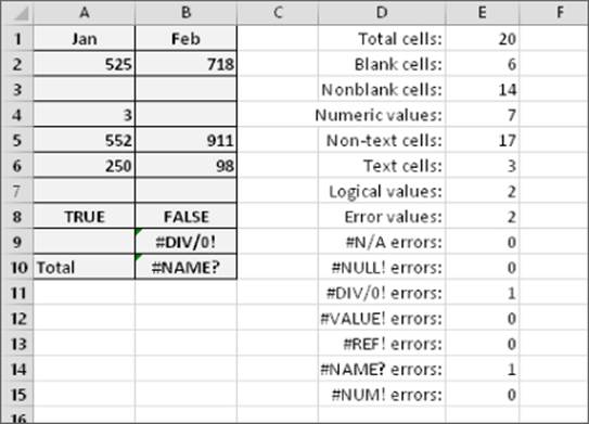
Figure 13.1 Formulas in column E display various counts of the data in A1:B10.

This workbook is available on this book's website at www.wiley.com/go/excel2016bible. The file is named basic counting.xlsx.

About This Chapter's Examples

Most of the examples in this chapter use named ranges for function arguments. When you adapt these formulas for your own use, you'll need to substitute either the actual range address or a range name defined in your workbook. (See Chapter 4, “Working with Cells and Ranges,” for information about using named ranges.)

Also, some examples consist of array formulas. An array formula is a special type of formula that enables you to perform calculations that would not otherwise be possible. You can spot an array formula because it's enclosed in curly brackets when it's displayed in the Formula bar. I use this syntax for the array formula examples presented in this book. For example:

{=Data*2}

When you enter an array formula, press Ctrl+Shift+Enter (not just Enter), but don't type the curly brackets. (Excel inserts the brackets for you.) If you need to edit an array formula, don't forget to press Ctrl+Shift+Enter when you finish editing; otherwise, the array formula will revert to a normal formula, and it will return an incorrect result. (See Chapter 17 for an introduction to array formulas.)

Counting the total number of cells

Oddly, Excel doesn't have a function that simply counts the number of cells in a range reference. To get a count of the total number of cells in a range (empty and nonempty cells), use the following formula. This formula returns the number of cells in a range named Data. It simply multiplies the number of rows (returned by the ROWS function) by the number of columns (returned by the COLUMNS function):

=ROWS(Data)*COLUMNS(Data)

This formula will not work if the Data range consists of noncontiguous cells. In other words, Data must be a rectangular range of cells.

Counting blank cells

The following formula returns the number of blank (empty) cells in a range named Data:

=COUNTBLANK(Data)

This function works only with a contiguous range of cells. If Data is defined as a noncontiguous range, the function returns a #VALUE! error.

The COUNTBLANK function also counts cells containing a formula that returns an empty string. For example, the formula that follows returns an empty string if the value in cell A1 is greater than 5. If the cell meets this condition, the COUNTBLANK function counts that cell:

=IF(A1>5,"",A1)

You can use the COUNTBLANK function with an argument that consists of entire rows or columns. For example, the following formula returns the number of blank cells in column A:

=COUNTBLANK(A:A)

The following formula returns the number of empty cells on the entire worksheet named Sheet1. You must enter this formula on a sheet other than Sheet1, or it will create a circular reference:

=COUNTBLANK(Sheet1!1:1048576)

Counting nonblank cells

To count nonblank cells, use the COUNTA function. The following formula uses the COUNTA function to return the number of nonblank cells in a range named Data:

=COUNTA(Data)

The COUNTA function counts cells that contain values, text, or logical values (TRUE or FALSE).

Note

If a cell contains a formula that returns an empty string, that cell is included in the count returned by COUNTA, even though the cell appears to be blank.

Counting numeric cells

To count only the numeric cells in a range, use the following formula (which assumes the range is named Data):

=COUNT(Data)

Cells that contain a date or a time are considered to be numeric cells. Cells that contain a logical value (TRUE or FALSE) aren't considered to be numeric cells.

Counting text cells

To count the number of text cells in a range, you need to use an array formula. The array formula that follows returns the number of text cells in a range named Data:

{=SUM(IF(ISTEXT(Data),1))}

Counting nontext cells

The following array formula uses the Excel ISNONTEXT function, which returns TRUE if its argument refers to any nontext cell (including a blank cell). This formula returns the count of the number of cells not containing text (including blank cells):

{=SUM(IF(ISNONTEXT(Data),1))}

Counting logical values

The following array formula returns the number of logical values (TRUE or FALSE) in a range named Data:

{=SUM(IF(ISLOGICAL(Data),1))}

Counting error values in a range

Excel has three functions that help you determine whether a cell contains an error value:

· ISERROR: Returns TRUE if the cell contains any error value (#N/A, #VALUE!, #REF!, #DIV/0!, #NUM!, #NAME?, or #NULL!)

· ISERR: Returns TRUE if the cell contains any error value except #N/A

· ISNA: Returns TRUE if the cell contains the #N/A error value

You can use these functions in an array formula to count the number of error values in a range. The following array formula, for example, returns the total number of error values in a range named Data:

{=SUM(IF(ISERROR(data),1))}

Depending on your needs, you can use the ISERR or ISNA function in place of ISERROR.

If you want to count specific types of errors, you can use the COUNTIF function. The following formula, for example, returns the number of #DIV/0! error values in the range named Data:

=COUNTIF(Data,"#DIV/0!")

Note that the COUNTIF functions works only with a contiguous range argument. If Data is a noncontiguous range, the formula returns a #VALUE! error.

Advanced Counting Formulas

Most of the basic examples I presented earlier in this chapter use functions or formulas that perform conditional counting. The advanced counting formulas that I present in this section represent more complex examples for counting worksheet cells, based on various types of criteria.

Some of these examples are array formulas. See Chapters 17 and 18 for more information about array formulas.

Counting cells by using the COUNTIF function

The COUNTIF function, which is useful for single-criterion counting formulas, takes two arguments:

· range: The range that contains the values that determine whether to include a particular cell in the count

· criteria: The logical criteria that determine whether to include a particular cell in the count

Table 13.2 lists several examples of formulas that use the COUNTIF function. All these formulas work with a range named Data. As you can see, the criteria argument proves quite flexible. You can use constants, expressions, functions, cell references, and even wildcard characters (* and ?).

Table 13.2 Examples of Formulas Using the COUNTIF Function

Note that the COUNTIF functions work only with a contiguous range argument. If Data is defined as a noncontiguous range, the formula returns a #VALUE! error.

Counting cells based on multiple criteria

In many cases, your counting formula will need to count cells only if two or more criteria are met. These criteria can be based on the cells that are being counted or on a range of corresponding cells.

Figure 13.2 shows a simple worksheet that I use for the examples in this section. This sheet shows sales data categorized by Month, Sales Rep, and Type. The worksheet contains four named ranges that correspond to the labels in row 1.

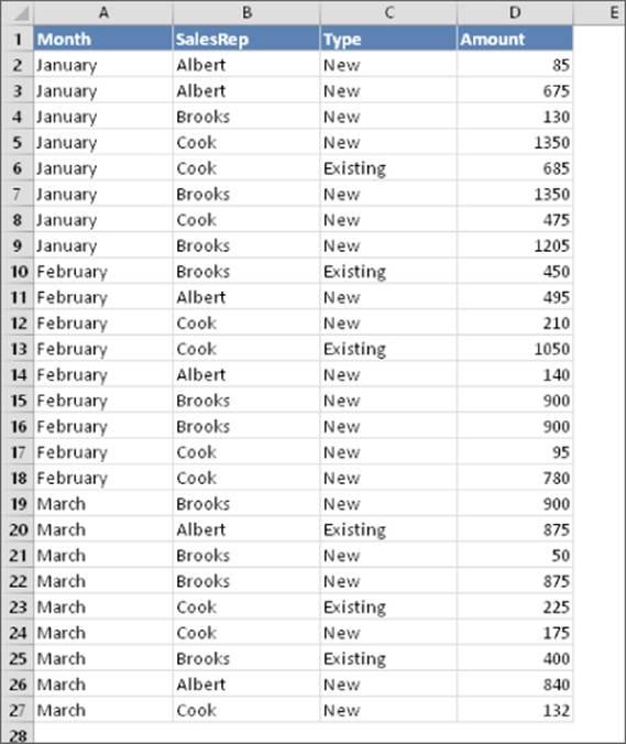
Figure 13.2 This worksheet demonstrates various counting techniques that use multiple criteria.

This workbook is available on this book's website at www.wiley.com/go/excel2016bible. The file is named multiple criteria counting.xlsx.

Note

Several of the examples in this section use the COUNTIFS function, which was introduced in Excel 2007. I also present alternative versions of the formulas, which you should use if you plan to share your workbook with others who use a version prior to Excel 2007.

Using And criteria

An And criterion counts cells if all specified conditions are met. A common example is a formula that counts the number of values that fall within a numerical range. For example, you may want to count cells that contain a value that's greater than 100 and less than or equal to 200. For this example, the COUNTIFS function will do the job:

=COUNTIFS(Amount,">100",Amount,"<=200")

Note

If the data is contained in a table, you can use table referencing in your formulas. For example, if the table is named Table1, you can rewrite the preceding formula as follows:

=COUNTIFS(Table1[Amount],">100",Table1[Amount],"<=200")

This method of writing formulas does not require named ranges. Excel automatically creates names for the table and each column in the table.

The COUNTIFS function accepts any number of paired arguments. The first member of the pair is the range to be counted (in this case, the range named Amount); the second member of the pair is the criterion. The preceding example contains two sets of paired arguments and returns the number of cells in which Amount is greater than 100 and less than or equal to 200.

Prior to Excel 2007, you would need to use a formula like this:

=COUNTIF(Amount,">100")-COUNTIF(Amount,">200")

This formula counts the number of values that are greater than 100 and then subtracts the number of values that are greater than or equal to 200. The result is the number of cells that contain a value greater than 100 and less than or equal to 200. This formula can be confusing because the formula refers to a condition ">200" even though the goal is to count values that are less than or equal to 200.

Yet another alternate technique is to use an array formula, like the one that follows. You may find it easier to create this type of formula:

{=SUM((Amount>100)*(Amount<=200))}

Note

When you enter an array formula, remember to press Ctrl+Shift+Enter, but don't type the curly brackets. Excel includes the brackets for you.

Sometimes the counting criteria will be based on cells other than the cells being counted. You may, for example, want to count the number of sales that meet all the following criteria:

· Month is January and

· SalesRep is Brooks and

· Amount is greater than 1,000

The following formula (for Excel 2007 and later) returns the number of items that meet all three criteria. Note that the COUNTIFS function uses three sets of paired arguments:

=COUNTIFS(Month,"January",SalesRep,"Brooks",Amount,">1000")

An alternative formula, which works with all versions of Excel, uses the SUMPRODUCT function. The following formula returns the same result as the previous formula:

=SUMPRODUCT((Month="January")*(SalesRep="Brooks")*(Amount>1000))

Yet another way to perform this count is to use an array formula:

{=SUM((Month="January")*(SalesRep="Brooks")*(Amount>1000))}

Using Or criteria

An Or criterion counts cells if any of the multiple conditions is met. To count cells by using an Or criterion, you can sometimes use multiple COUNTIF functions. The following formula, for example, counts the number of sales made in January or February:

=COUNTIF(Month,"January")+COUNTIF(Month,"February")

You can also use the COUNTIF function in an array formula. The following array formula, for example, returns the same result as the previous formula:

{=SUM(COUNTIF(Month,{"January","February"}))}

But if you base your Or criteria on cells other than the cells being counted, the COUNTIF function won't work (refer to Figure 13.2). Suppose that you want to count the number of sales that meet at least one of the following criteria:

· Month is January or

· SalesRep is Brooks or

· Amount is greater than 1,000

If you attempt to create a formula that uses COUNTIF, some double counting will occur. The solution is to use an array formula like this:

{=SUM(IF((Month="January")+(SalesRep="Brooks")+(Amount>1000),1))}

Combining And and Or criteria

In some cases, you may need to combine And criteria and Or criteria when counting. For example, perhaps you want to count sales that meet both of the following criteria:

· Month is January.

· SalesRep is Brooks or SalesRep is Cook.

This array formula returns the number of sales that meet the criteria:

{=SUM((Month="January")*IF((SalesRep="Brooks")+(SalesRep="Cook"),1))}

Counting the most frequently occurring entry

The MODE function returns the most frequently occurring value in a range. In case of a tie, it returns the mode of the value that appears first in the range. Figure 13.3 shows a worksheet with values in range A1:A10 (named Data). The formula that follows returns 10because that value appears most frequently in the Data range:

=MODE(Data)

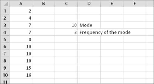
Figure 13.3 The MODE function returns the most frequently occurring value in a range.

To count the number of times the most frequently occurring value appears in the range (in other words, the frequency of the mode), use the following formula:

=COUNTIF(Data,MODE(Data))

This formula returns 3 because the modal value (10) appears three times in the Data range.

The MODE function works only for numeric values. It simply ignores cells that contain text. To find the most frequently occurring text entry in a range, you need to use an array formula.

To count the number of times the most frequently occurring item (text or values) appears in a range named Data, use the following array formula:

{=MAX(COUNTIF(Data,Data))}

This next array formula operates like the MODE function except that it works with both text and values:

{=INDEX(Data,MATCH(MAX(COUNTIF(Data,Data)),COUNTIF(Data,Data),0))}

Counting the occurrences of specific text

The examples in this section demonstrate various ways to count the occurrences of a character or text string in a range of cells. Figure 13.4 shows a worksheet used for these examples. Various text strings appear in the range A1:A10 (named Data); cell B1 is named Text.

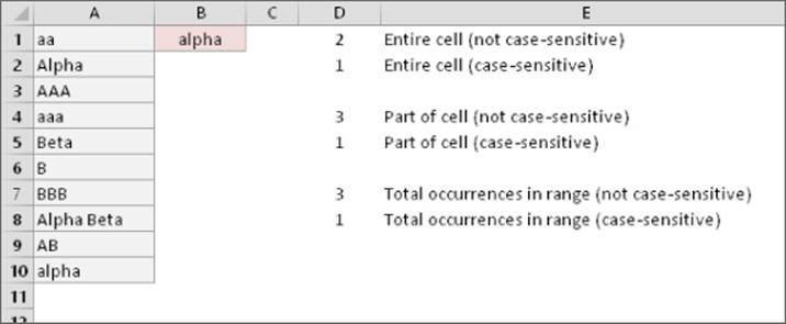
Figure 13.4 This worksheet demonstrates various ways to count character strings in a range.

This book's website at www.wiley.com/go/excel2016bible contains a workbook that demonstrates the formulas in this section. The file is named counting text in a range.xlsx.

Entire cell contents

To count the number of cells containing the contents of the Text cell (and nothing else), you can use the COUNTIF function as the following formula demonstrates:

=COUNTIF(Data,Text)

For example, if the Text cell contains the string Alpha, the formula returns 2 because two cells in the Data range contain this text. This formula is not case sensitive, so it counts both Alpha (cell A2) and alpha (cell A10). Note, however, that it does not count the cell that contains Alpha Beta (cell A8).

The following array formula is similar to the preceding formula, but this one is case sensitive:

{=SUM(IF(EXACT(Data,Text),1))}

Partial cell contents

To count the number of cells that contain a string that includes the contents of the Text cell, use this formula:

=COUNTIF(Data,"*"&Text&"*")

For example, if the Text cell contains the text Alpha, the formula returns 3 because three cells in the Data range contain the text alpha (cells A2, A8, and A10). Note that the comparison is not case sensitive.

If you need a case-sensitive count, you can use the following array formula:

{=SUM(IF(LEN(Data)-LEN(SUBSTITUTE(Data,Text,""))>0,1))}

If the Text cells contain the text Alpha, the preceding formula returns 2 because the string appears in two cells (A2 and A8).

Total occurrences in a range

To count the total number of occurrences of a string within a range of cells, use the following array formula:

{=(SUM(LEN(Data))-SUM(LEN(SUBSTITUTE(Data,Text,""))))/LEN(Text)}

If the Text cell contains the character B, the formula returns 7 because the range contains seven instances of the string. This formula is case sensitive.

The following array formula is a modified version that is not case sensitive:

{=(SUM(LEN(Data))-SUM(LEN(SUBSTITUTE(UPPER(Data),UPPER(Text),""))))/LEN(Text)}

Counting the number of unique values

The following array formula returns the number of unique values in a range named Data:

{=SUM(1/COUNTIF(Data,Data))}

Note

The preceding formula is one of those “classic” Excel formulas that gets passed around on the Internet. I don't know who originated it.

Useful as it is, this formula does have a serious limitation: if the range contains any blank cells, it returns an error. The following array formula solves this problem:

{=SUM(IF(COUNTIF(Data,Data)=0,"",1/COUNTIF(Data,Data)))}

To find out how to create a multicell array formula that returns a list of unique items in a range, see Chapter 18.

This book's website at www.wiley.com/go/excel2016bible contains a workbook that demonstrates this technique. The file is named count unique.xlsx.

Creating a frequency distribution

A frequency distribution is a summary table that shows the frequency of each value in a range. For example, an instructor may create a frequency distribution of grades. The table would show the count of As, Bs, Cs, and so on. Excel provides a number of ways to create frequency distributions. You can

· Use the FREQUENCY function.

· Create your own formulas.

· Use the Analysis ToolPak add-in.

· Use a pivot table.

Excel 2016 includes a new Histogram chart feature, which can create a frequency histogram from a set of values. This feature does not create a table, however. For an example of a histogram chart, see Chapter 19, “Getting Started Making Charts.”

A workbook that demonstrates these four techniques is available on this book's website at www.wiley.com/go/excel2016bible. The file is named frequency distribution.xlsx.

The FREQUENCY function

Using the FREQUENCY function to create a frequency distribution can be a bit tricky; it is probably the most difficult way to create a frequency distribution. The FREQUENCY function always returns an array, so you must use it in an array formula that's entered into a multicell range.

Figure 13.5 shows some data in range A1:E25 (named Data). These values range from 1 to 500. The range G2:G11 contains the bins used for the frequency distribution. Each cell in this bin range contains the upper limit for the bin. In this case, the bins consist of <=50, 51–100, 101–150, and so on. The goal is to count the number of values that fall into each bin.

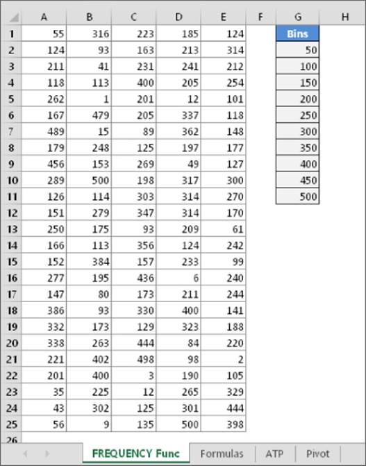
Figure 13.5 Creating a frequency distribution for the data in A1:E25.

To create the frequency distribution, select a range of cells that corresponds to the number of cells in the bin range. (In this example, select H2:H11 because the bins are in G2:G11.) Then enter the following array formula into the selected range. (Press Ctrl+Shift+Enter to enter an array formula.)

{=FREQUENCY(Data,G2:G11)}

The array formula returns the count of values in the Data range that fall into each bin. To create a frequency distribution that consists of percentages, use the following array formula:

{=FREQUENCY(Data,G2:G11)/COUNT(Data)}

Figure 13.6 shows two frequency distributions — one in terms of counts and one in terms of percentages. The figure also shows a chart (histogram) created from the frequency distribution.

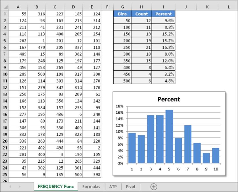
Figure 13.6 Frequency distributions created by using the FREQUENCY function.

Using formulas to create a frequency distribution

Figure 13.7 shows a worksheet that contains test scores for 50 students in column B (the range is named Grades). Formulas in columns G and H calculate a frequency distribution for letter grades. The minimum and maximum values for each letter grade appear in columns D and E. For example, a test score between 80 and 89 (inclusive) earns a B. In addition, a chart displays the distribution of the test scores.

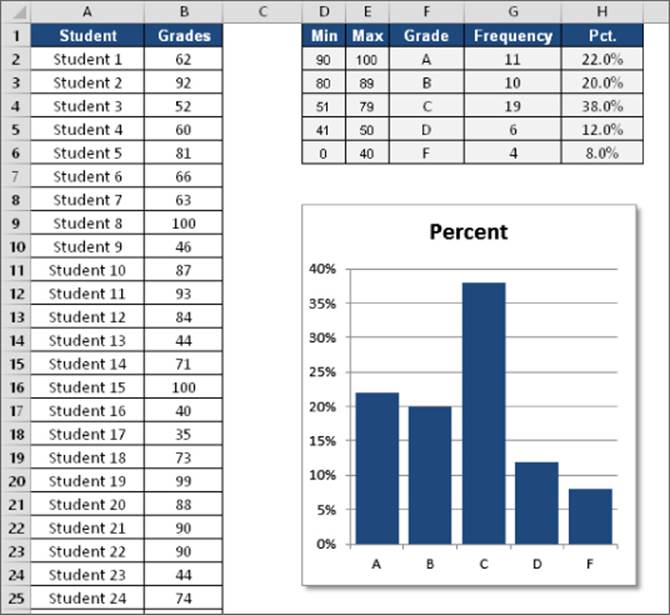
Figure 13.7 Creating a frequency distribution of test scores.

The formula in cell G2 that follows counts the number of scores that qualify for an A:

=COUNTIFS(Grades,">="&D2,Grades,"<="&E2)

You may recognize this formula from a previous section in this chapter (see “Counting cells based on multiple criteria”). This formula was copied to the four cells below G2.

Note

The preceding formula uses the COUNTIFS function, which first appeared in Excel 2007. For compatibility with previous Excel versions, use this array formula:

{=SUM((Grades>=D2)*(Grades<=E2))}

The formulas in column H calculate the percentage of scores for each letter grade. The formula in H2, which was copied to the four cells below H2, is

=G2/SUM($G$2:$G$6)

Using the Analysis ToolPak to create a frequency distribution

The Analysis ToolPak add-in, distributed with Excel, provides another way to calculate a frequency distribution:

1. Enter your bin values in a range.

2. Choose Data Analysis Analysis. The Data Analysis dialog box appears. If this command is not available, see the next sidebar, “Is the Analysis ToolPak Installed?”

3. In the Data Analysis dialog box, select Histogram, and then click OK. The Histogram dialog box, shown in Figure 13.8, appears.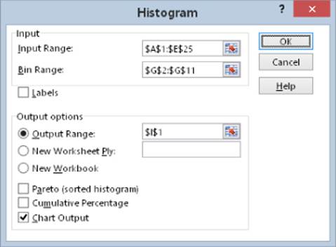

Figure 13.8 The Analysis ToolPak's Histogram dialog box.

4. Specify the ranges for your data (Input Range), bins (Bin Range), and results (Output Range), and then select any options and click OK. Figure 13.9 shows a frequency distribution (and chart) created with the Histogram option.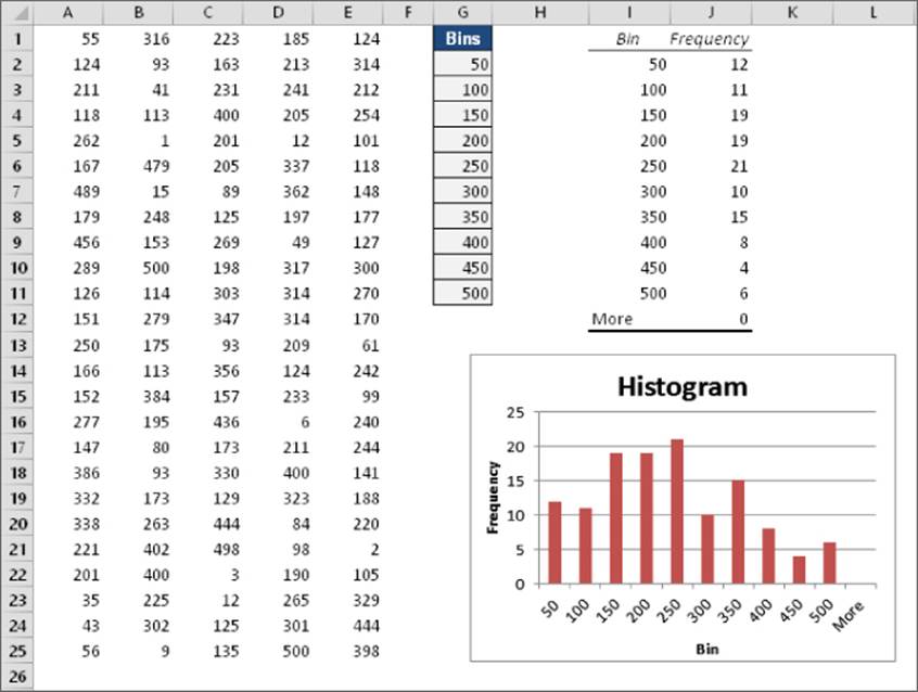

Figure 13.9 A frequency distribution and chart generated by the Analysis ToolPak's Histogram option.

Caution

Note that the frequency distribution consists of values, not formulas. Therefore, if you make any changes to your input data, you need to rerun the Histogram procedure to update the results.

Is the Analysis ToolPak Installed?

To make sure that the Analysis ToolPak add-in is installed, click the Data tab. If the Ribbon displays the Data Analysis command in the Analysis group, you're all set. If not, you'll need to install the add-in:

1. Choose File Options. The Excel Options dialog box appears.

2. Click the Add-ins tab on the left.

3. Select Excel Add-Ins from the Manage drop-down list.

4. Click Go to display the Add-Ins dialog box.

5. Place a check mark next to Analysis ToolPak.

6. Click OK.

If you've enabled the Developer tab, you can display the Add-Ins dialog box by choosing Developer Add-Ins Add-Ins.

Note: In the Add-Ins dialog box, you see an additional add-in, Analysis ToolPak – VBA. This add-in is for programmers; you don't need to install it.

Using a pivot table to create a frequency distribution

If your data is in the form of a table, you may prefer to use a pivot table and a pivot chart to create a histogram. Figure 13.10 shows the student grade data summarized in a pivot table (in D1:E9) and a pivot chart. The counts were created by grouping.

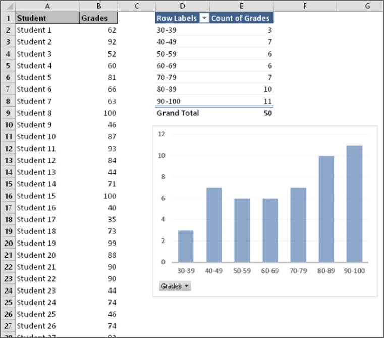
Figure 13.10 Using a pivot chart to display a histogram.

I cover pivot tables in detail in Chapter 33, “Introducing Pivot Tables,” and Chapter 34, “Analyzing Data with Pivot Tables.”

Summing Formulas

The examples in this section demonstrate how to perform common summing tasks by using formulas. The formulas range from simple to relatively complex array formulas that compute sums by using multiple criteria.

Summing all cells in a range

It doesn't get much simpler than this. The following formula returns the sum of all values in a range named Data:

=SUM(Data)

The SUM function can take up to 255 arguments. The following formula, for example, returns the sum of the values in five noncontiguous ranges:

=SUM(A1:A9,C1:C9,E1:E9,G1:G9,I1:I9)

You can use complete rows or columns as an argument for the SUM function. The formula that follows, for example, returns the sum of all values in column A. If this formula appears in a cell in column A, it generates a circular reference error:

=SUM(A:A)

The following formula returns the sum of all values on Sheet1 by using a range reference that consists of all rows. To avoid a circular reference error, this formula must appear on a sheet other than Sheet1:

=SUM(Sheet1!1:1048576)

The SUM function is versatile. The arguments can be numerical values, cells, ranges, text representations of numbers (which are interpreted as values), logical values, and even embedded functions. For example, consider the following formula:

=SUM(B1,5,"6",,SQRT(4),A1:A5,TRUE)

This odd formula, which is perfectly valid, contains all the following types of arguments, listed here in the order of their presentation:

· A single cell reference: B1

· A literal value: 5

· A string that looks like a value: "6"

· A missing argument: , ,

· An expression that uses another function: SQRT(4)

· A range reference: A1:A5

· A logical value: TRUE

Caution

The SUM function is versatile, but it's also inconsistent when you use logical values (TRUE or FALSE). Logical values stored in cells are always treated as 0. However, logical TRUE, when used as an argument in the SUM function, is treated as 1.

Computing a cumulative sum

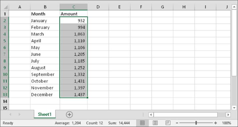
You may want to display a cumulative sum of values in a range — sometimes known as a “running total.” Figure 13.11 illustrates a cumulative sum. Column B shows the monthly amounts, and column C displays the cumulative (year-to-date) totals.

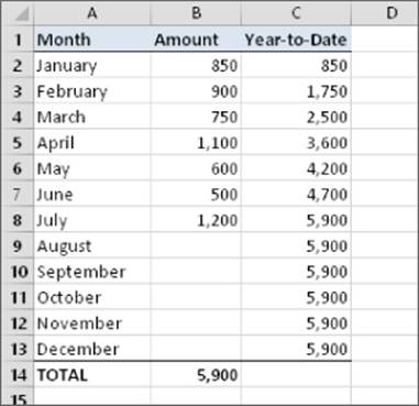
Figure 13.11 Simple formulas in column C display a cumulative sum of the values in column B.

The formula in cell C2 is

=SUM(B$2:B2)

Notice that this formula uses a mixed reference — that is, the first cell in the range reference always refers to the same row (in this case, row 2). When this formula is copied down the column, the range argument adjusts such that the sum always starts with row 2 and ends with the current row. For example, after copying this formula down column C, the formula in cell C8 is

=SUM(B$2:B8)

You can use an IF function to hide the cumulative sums for rows in which data hasn't been entered. The following formula, entered into cell C2 and copied down the column, is

=IF(B2<>"",SUM(B$2:B2),"")

Figure 13.12 shows this formula at work.

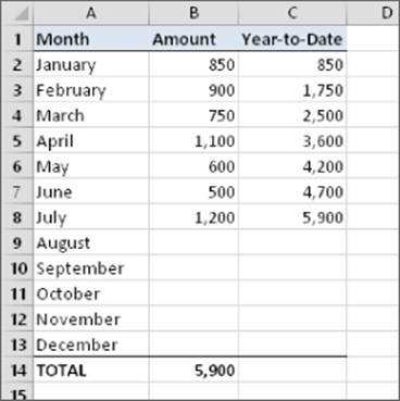
Figure 13.12 Using an IF function to hide cumulative sums for missing data.

This workbook is available on this book's website at www.wiley.com/go/excel2016bible. The file is named cumulative sum.xlsx.

Ignoring errors when summing

The SUM function does not work if the range to be summed includes errors. For example, if one of the cells to be summed displays #N/A, the SUM function will also return #N/A.

To add the values in a range and ignore the error cells, use the AGGREGATE function. For example, to sum a range named Data (which may have error values), use this formula:

=AGGREGATE(9,6,Data)

The AGGREGATE function is versatile and can do a lot more than just add values. In this example, the first argument (9) specifies SUM. The second argument (6) means ignore error values.

The arguments are described in the Excel Help. Excel also provides good autocomplete assistance when you enter a formula that uses this function.

Caution

The AGGREGATE function was introduced in Excel 2010. For compatibility with earlier versions, use this array formula:

{=SUM(IF(ISERROR(Data),"",Data))}

Summing the “top n” values

In some situations, you may need to sum the n largest values in a range — for example, the top ten values. If your data resides in a table, you can use autofiltering to hide all but the top n rows and then display the sum of the visible data in the table's total row.

Another approach is to sort the range in descending order and then use the SUM function with an argument consisting of the first n values in the sorted range.

A better solution — which doesn't require a table or sorting — uses an array formula like this one:

{=SUM(LARGE(Data,{1,2,3,4,5,6,7,8,9,10}))}

This formula sums the ten largest values in a range named Data. To sum the ten smallest values, use the SMALL function instead of the LARGE function:

{=SUM(SMALL(Data,{1,2,3,4,5,6,7,8,9,10}))}

These formulas use an array constant composed of the arguments for the LARGE or SMALL function. If the value of n for your top-n calculation is large, you may prefer to use the following variation. This formula returns the sum of the top 20 values in the Data range. You can, of course, substitute a different value for 20. Figure 13.13 shows this array formula in use.

{=SUM(LARGE(Data,ROW(INDIRECT("1:20"))))}

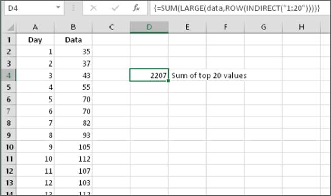
Figure 13.13 Using an array formula to calculate the sum of the 20 largest values in a range.

See Chapter 17 for more information about using array constants.

Conditional Sums Using a Single Criterion

Often, you need to calculate a conditional sum. With a conditional sum, values in a range that meet one or more conditions are included in the sum. This section presents examples of conditional summing by using a single criterion.

The SUMIF function is useful for single-criterion sum formulas. The SUMIF function takes three arguments:

· range: The range containing the values that determine whether to include a particular cell in the sum.

· criteria: An expression that determines whether to include a particular cell in the sum.

· sum_range: Optional. The range that contains the cells you want to sum. If you omit this argument, the function uses the range specified in the first argument.

The examples that follow demonstrate the use of the SUMIF function. These formulas are based on the worksheet shown in Figure 13.14, set up to track invoices. Column F contains a formula that subtracts the date in column E from the date in column D. A negative number in column F indicates a past-due payment. The worksheet uses named ranges that correspond to the labels in row 1.

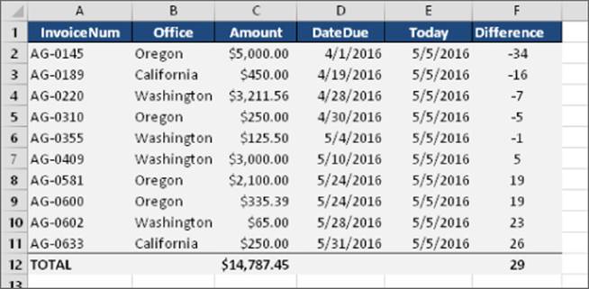
Figure 13.14 A negative value in column F indicates a past-due payment.

All the examples in this section are available at this book's website at www.wiley.com/go/excel2016bible. The file is named conditional sum.xlsx.

Summing only negative values

The following formula returns the sum of the negative values in column F. In other words, it returns the total number of past-due days for all invoices. For this worksheet, the formula returns –63.

=SUMIF(Difference,"<0")

Because you omit the third argument, the second argument ("<0") applies to the values in the Difference range.

You don't need to hard-code the arguments for the SUMIF function into your formula. For example, you can create a formula, such as the following, which gets the criteria argument from the contents of cell G2:

=SUMIF(Difference,G2)

This formula returns a new result if you change the criteria in cell G2.

Summing values based on a different range

The following formula returns the sum of the past-due invoice amounts (in column C):

=SUMIF(Difference,"<0",Amount)

This formula uses the values in the Difference range to determine whether the corresponding values in the Amount range contribute to the sum.

Summing values based on a text comparison

The following formula returns the total invoice amounts for the Oregon office:

=SUMIF(Office,"=Oregon",Amount)

Using the equal sign in the argument is optional. The following formula has the same result:

=SUMIF(Office,"Oregon",Amount)

To sum the invoice amounts for all offices except Oregon, use this formula:

=SUMIF(Office,"<>Oregon",Amount)

Summing values based on a date comparison

The following formula returns the total invoice amounts that have a due date after May 1, 2016:

=SUMIF(DateDue,">="&DATE(2016,5,1),Amount)

Notice that the second argument for the SUMIF function is an expression. The expression uses the DATE function, which returns a date. Also, the comparison operator, enclosed in quotes, is concatenated (using the & operator) with the result of the DATE function.

The formula that follows returns the total invoice amounts that have a future due date (including today):

=SUMIF(DateDue,">="&TODAY(),Amount)

Conditional Sums Using Multiple Criteria

All the examples in the preceding section used a single comparison criterion. The examples in this section involve summing cells based on multiple criteria.

Figure 13.15 shows the sample worksheet again, for your reference. The worksheet also shows the result of several formulas that demonstrate summing by using multiple criteria.

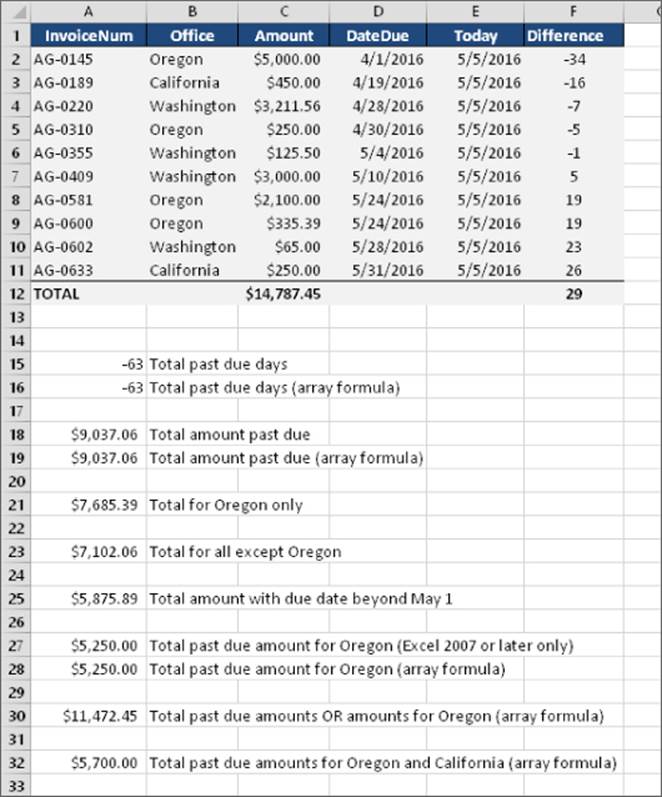
Figure 13.15 This worksheet demonstrates summing based on multiple criteria.

Using And criteria

Suppose that you want to get a sum of the invoice amounts that are past due and associated with the Oregon office. In other words, the value in the Amount range will be summed only if both of the following criteria are met:

· The corresponding value in the Difference range is negative, and

· The corresponding text in the Office range is Oregon.

If the worksheet won't be used by anyone running a version prior to Excel 2007, the following formula does the job:

=SUMIFS(Amount,Difference,"<0",Office,"Oregon")

The following array formula returns the same result and will work in all versions of Excel:

{=SUM((Difference<0)*(Office="Oregon")*Amount)}

Using Or criteria

Suppose that you want to get a sum of past-due invoice amounts or ones associated with the Oregon office. In other words, the value in the Amount range will be summed if either of the following criteria is met:

· The corresponding value in the Difference range is negative.

· The corresponding text in the Office range is Oregon.

This example requires an array formula:

{=SUM(IF((Office="Oregon")+(Difference<0),1,0)*Amount)}

A plus sign (+) joins the conditions; you can include more than two conditions.

Using And and Or criteria

As you may expect, things get a bit tricky when your criteria consists of both And and Or operations. For example, you may want to sum the values in the Amount range when both of the following conditions are met:

· The corresponding value in the Difference range is negative.

· The corresponding text in the Office range is Oregon or California.

Notice that the second condition actually consists of two conditions joined with Or. The following array formula does the trick:

{=SUM((Difference<0)*IF((Office="Oregon")+(Office="California"),1)*Amount)}