Microsoft Excel 2016 BIBLE (2016)

IN THIS CHAPTER

1. Getting a brief overview of the Excel functions that deal with the time value of money

2. Looking at formulas that perform various types of loan calculations

3. Considering formulas that perform various types of investment calculations

4. Reviewing Excel depreciation functions

5. Using the new forecasting functions

It's a safe bet that the most common use of Excel is to perform calculations involving money. Every day, people make hundreds of thousands of financial decisions based on the numbers that are calculated in a spreadsheet. These decisions range from simple (“Can I afford to buy a new car?”) to complex (“Will purchasing XYZ Corporation result in a positive cash flow in the next 18 months?”). This chapter discusses basic financial calculations that you can perform with the assistance of Excel.

The Time Value of Money

The face value of money may not always be what it seems. A key consideration is the time value of money. This concept involves calculating the value of money in the past, present, or future. It's based on the premise that money increases in value over time because of interest earned by the money. In other words, a dollar invested today will be worth more tomorrow.

For example, imagine that your rich uncle decided to give away some money and asked you to choose one of the following options:

· Receive $8,000 today.

· Receive $9,500 in one year.

· Receive $12,000 in five years.

· Receive $150 per month for five years.

If your goal is to maximize the amount received, you need to take into account not only the face value of the money but also the time value of the money when it arrives in your hands.

The time value of money depends on your perspective. In other words, you're either a lender or a borrower. When you take out a loan to purchase an automobile, you're a borrower, and the institution that provides the funds to you is the lender. When you invest money in a bank savings account, you're a lender; you're lending your money to the bank, and the bank is borrowing it from you.

Several concepts contribute to the time value of money:

· Present value (PV): This is the principal amount. If you deposit $5,000 in a bank savings account, this amount represents the principal, or present value, of the money you invested. If you borrow $15,000 to purchase a car, this amount represents the principal, or present value, of the loan. Present value may be positive or negative.

· Future value (FV): This is the principal plus interest. If you invest $5,000 for five years and earn 3% annual interest, your investment is worth $5,796.37 at the end of the five-year term. This amount is the future value of your $5,000 investment. If you take out a three-year car loan for $15,000 and make monthly payments based on a 5.25% annual interest rate, you pay a total of $16,244.97. This amount represents the principal plus the interest you paid. Future value may be positive or negative, depending on the perspective (lender or borrower).

· Payment (PMT): This is either principal or principal plus interest. If you deposit $100 per month into a savings account, $100 is the payment. If you have a monthly mortgage payment of $1,025, this amount is made up of principal and interest.

· Interest rate: Interest is a percentage of the principal, usually expressed on an annual basis. For example, you may earn 2.5% annual interest on a bank CD (certificate of deposit). Or your mortgage loan may have a 6.75% interest rate.

· Period: This represents the point in time when interest is paid or earned (for example, a bank CD that pays interest quarterly, or an auto loan that requires monthly payments).

· Term: This is the amount of time of interest. A 12-month bank CD has a term of one year. A 30-year mortgage loan has a term of 360 months.

Loan Calculations

This section describes how to calculate various components of a loan. Think of a loan as consisting of the following components:

· The loan amount

· The interest rate

· The number of payment periods

· The periodic payment amount

If you know any three of these components, you can create a formula to calculate the unknown component.

Note

The loan calculations in this section all assume a fixed-rate loan with a fixed term.

Worksheet functions for calculating loan information

This section describes six commonly used financial functions: PMT, PPMT, IPMT, RATE, NPER, and PV. For information about the arguments used in these functions, see Table 15.1.

Table 15.1 Financial Function Arguments

PMT

The PMT function returns the loan payment (principal plus interest) per period, assuming constant payment amounts and a fixed interest rate. The syntax for the PMT function follows:

PMT(rate,nper,pv,fv,type)

The following formula returns the monthly payment amount for a $5,000 loan with a 6% annual percentage rate. The loan has a term of four years (48 months).

=PMT(6%/12,48,-5000)

This formula returns $117.43, the monthly payment for the loan. The first argument, rate, is the annual rate divided by the number of months in a year. Also, notice that the third argument (pv, for present value) is negative and represents money owed.

PPMT

The PPMT function returns the principal part of a loan payment for a given period, assuming constant payment amounts and a fixed interest rate. The syntax for the PPMT function is

PPMT(rate,per,nper,pv,fv,type)

The following formula returns the amount paid to principal for the first month of a $5,000 loan with a 6% annual percentage rate. The loan has a term of four years (48 months).

=PPMT(6%/12,1,48,-5000)

The formula returns $92.43 for the principal, which is about 78.7% of the total loan payment. If I change the second argument to 48 (to calculate the principal amount for the last payment), the formula returns $116.84, or about 99.5% of the total loan payment.

Note

To calculate the cumulative principal paid between any two payment periods, use the CUMPRINC function. This function uses two additional arguments: start_period and end_period. In Excel versions prior to Excel 2007, CUMPRINC is available only when you install the Analysis ToolPak add-in.

IPMT

The IPMT function returns the interest part of a loan payment for a given period, assuming constant payment amounts and a fixed interest rate. The syntax for the IPMT function is

IPMT(rate,per,nper,pv,fv,type)

The following formula returns the amount paid to interest for the first month of a $5,000 loan with a 6% annual percentage rate. The loan has a term of four years (48 months).

=IPMT(6%/12,1,48,-5000)

This formula returns an interest amount of $25.00. By the last payment period for the loan, the interest payment is only $0.58.

Note

To calculate the cumulative interest paid between any two payment periods, use the CUMIPMT function. This function uses two additional arguments: start_period and end_period. In Excel versions prior to Excel 2007, CUMIPMT is available only when you install the Analysis ToolPak add-in.

RATE

The RATE function returns the periodic interest rate of a loan, given the number of payment periods, the periodic payment amount, and the loan amount. The syntax for the RATE function is

RATE(nper,pmt,pv,fv,type,guess)

The following formula calculates the annual interest rate for a 48-month loan for $5,000 that has a monthly payment amount of $117.43:

=RATE(48,117.43,-5000)*12

This formula returns 6.00%. Notice that the result of the function is multiplied by 12 to get the annual percentage rate.

NPER

The NPER function returns the number of payment periods for a loan, given the loan's amount, interest rate, and periodic payment amount. The syntax for the NPER function is

NPER(rate,pmt,pv,fv,type)

The following formula calculates the number of payment periods for a $5,000 loan that has a monthly payment amount of $117.43. The loan has a 6% annual interest rate:

=NPER(6%/12,117.43,-5000)

This formula returns 47.997 (that is, 48 months). The monthly payment was rounded to the nearest penny, causing the minor discrepancy.

PV

The PV function returns the present value (that is, the original loan amount) for a loan, given the interest rate, the number of periods, and the periodic payment amount. The syntax for the PV function is

PV(rate,nper,pmt,fv,type)

The following formula calculates the original loan amount for a 48-month loan that has a monthly payment amount of $117.43. The annual interest rate is 6%.

=PV(6%/12,48,-117.43)

This formula returns $5,000.21. The monthly payment was rounded to the nearest penny, causing the $0.21 discrepancy.

A loan calculation example

Figure 15.1 shows a worksheet set up to calculate the periodic payment amount for a loan.

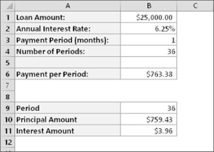
Figure 15.1 Using the PMT function to calculate a periodic loan payment amount.

The workbook described in this section is available on this book's website at www.wiley.com/go/excel2016bible. The file is named loan payment.xlsx.

The loan amount is in cell B1, and the annual interest rate is in cell B2. Cell B3 contains the payment period expressed in months. For example, if cell B3 is 1, the payment is due monthly. If cell B3 is 3, the payment is due every three months, or quarterly. Cell B4 contains the number of periods of the loan. The example shown in this figure calculates the payment for a $25,000 loan at 6.25% annual interest with monthly payments for 36 months. The formula in cell B6 is

=PMT(B2*(B3/12),B4,-B1)

Notice that the first argument is an expression that calculates the periodic interest rate by using the annual interest rate and the payment period. Therefore, if payments are made quarterly on a three-year loan, the payment period is 3, the number of periods is 12, and the periodic interest rate would be calculated as the annual interest rate multiplied by ³/₁₂.

In the worksheet in Figure 15.1, range A9:B11 is set up to calculate the principal and interest amount for a particular payment period. Cell B9 contains the payment period used by the formulas in B10:B11. (The payment period must be less than or equal to the value in cell B4.)

The formula in cell B10, shown here, calculates the amount of the payment that goes toward principal for the payment period in cell B9:

=PPMT(B2*(B3/12),B9,B4,-B1)

The following formula, in cell B11, calculates the amount of the payment that goes toward interest for the payment period in cell B9:

=IPMT(B2*(B3/12),B9,B4,-B1)

The sum of B10 and B11 is equal to the total loan payment calculated in cell B6. However, the relative proportion of principal and interest amounts varies with the payment period. (An increasingly larger proportion of the payment is applied toward principal as the loan progresses.) Figure 15.2 shows the principal and interest portions graphically.

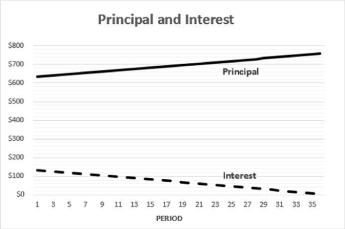
Figure 15.2 This chart shows how the interest and principal amounts vary during the payment periods of a loan.

Credit card payments

Do you ever wonder how long it would take to pay off a credit card balance if you make the minimum payment amount each month? Figure 15.3 shows a worksheet set up to make this type of calculation.

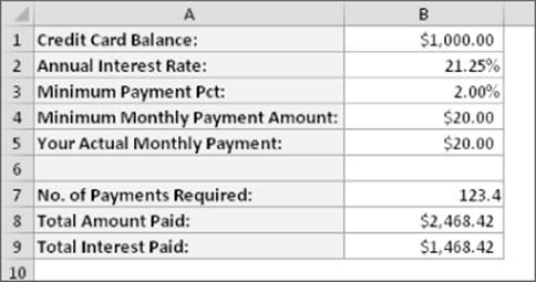
Figure 15.3 This worksheet calculates the number of payments required to pay off a credit card balance by paying the minimum payment amount each month.

The workbook shown in Figure 15.3 is available on this book's website at www.wiley.com/go/excel2016bible. The file is named credit card payments.xlsx.

Range B1:B5 stores input values. In this example, the credit card has a balance of $1,000, and the lender charges a 21.25% annual percentage rate (APR). The minimum payment is 2.00% (typical of many credit card lenders). Therefore, the minimum payment amount for this example is $20. You can enter a different payment amount in cell B5, but it must be large enough to pay off the loan. For example, you may choose to pay $50 per month to pay off the balance more quickly. However, paying $10 per month isn't sufficient, and the formulas return an error.

Range B7:B9 holds formulas that perform various calculations. The formula in cell B7, which follows, calculates the number of months required to pay off the balance:

=NPER(B2/12,B5,-B1,0)

The formula in B8 calculates the total amount you will pay. This formula is

=B7*B5

The formula in cell B9 calculates the total interest paid:

=B8-B1

In this example, it would take about 123 months (more than ten years) to pay off the credit card balance if the borrower made only the minimum monthly payment. The total interest paid on the $1,000 loan would be $1,468.42. This calculation assumes, of course, that no additional charges are made on the account. This example may help explain why you receive so many credit card solicitations in the mail.

Figure 15.4 shows some additional calculations for the credit card example. For example, if you want to pay off the credit card in 12 months, you need to make monthly payments of $93.23. (This amount results in total payments of $1,118.81 with total interest of $118.81.) The formula in B13 is

=PMT($B$2/12,A13,-$B$1)

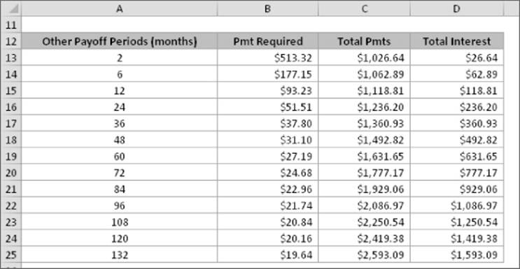
Figure 15.4 Column B shows the payment required to pay off the credit card balance for various payoff periods.

Creating a loan amortization schedule

A loan amortization schedule is a table of values that shows various types of information for each payment period of a loan. Figure 15.5 shows a worksheet that uses formulas to calculate an amortization schedule.

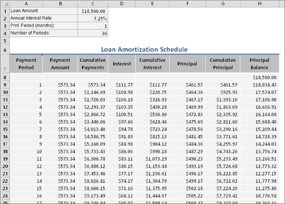
Figure 15.5 A loan amortization schedule.

This workbook is available on this book's website at www.wiley.com/go/excel2016bible. The file is named loan amortization schedule.xlsx.

The loan parameters are entered into C1:C4, and the formulas beginning in row 9 use these values for the calculations. Table 15.2 shows the formulas in row 9 of the schedule. These formulas were copied down to row 488. Therefore, the worksheet can calculate amortization schedules for a loan with as many as 480 payment periods (40 years of monthly payments).

Table 15.2 Formulas Used to Calculate an Amortization Schedule

Note

Formulas in the rows that extend beyond the number of payments return an error value. The worksheet uses conditional formatting to hide the data in these rows.

See Chapter 21, “Visualizing Data Using Conditional Formatting,” for more information about conditional formatting.

Summarizing loan options by using a data table

The Excel Data Table feature is probably one of the most underutilized tools in Excel. Keep in mind that a data table is not the same as a table (created by choosing Insert Tables Table). A data table is a handy way to summarize calculations that depend on one or two “changing” cells. In this example, I use a data table to summarize various loan options. This section describes how to create one-way and two-way data tables.

See Chapter 35, “Performing Spreadsheet What-If Analysis,” for more information about setting up data tables.

A workbook that demonstrates one- and two-way data tables is available on this book's website at www.wiley.com/go/excel2016bible. The file is named loan data tables.xlsx.

Creating a one-way data table

A one-way data table shows the results of any number of calculations for different values of a single input cell.

Figure 15.6 shows a one-way data table (in B10:I13) that displays three calculations (payment amount, total payments, and total interest) for a loan, using seven interest rates ranging from 7.00% to 8.50%. In this example, the input cell is cell B2.

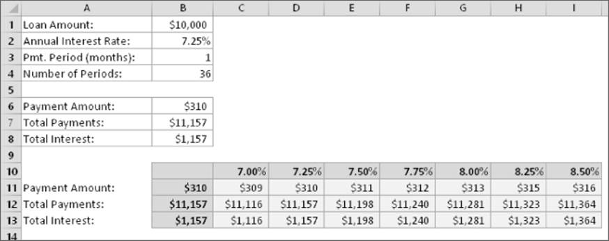
Figure 15.6 Using a one-way data table to display three loan calculations for various interest rates.

To create this one-way data table, follow these steps:

1. Enter the formulas that return the results for use in the data table. In this example, the formulas are in B6:B8.

2. Enter various values for a single input cell in successive columns. In this example, the input value is interest rate, and the values for various interest rates appear in C10:I10.

3. Create a reference to the formula cells in the column to the left of the input values. In this example, the range B11:B13 contains simple formulas that reference other cells. For example, cell B11 contains the following formula:

=B6

4. Select the rectangular range that contains the entries from the previous steps. In this example, select B10:I13.

5. Choose Data Data Tools What-If Analysis Data Table. The Data Table dialog box, shown in Figure 15.7, appears.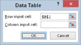

Figure 15.7 The Data Table dialog box.

6. For the Row input cell field, specify the cell reference that corresponds to the variable in your Data Table column header row. In this example, the Row input cell is B2.

7. Leave the Column input cell field empty. The Column input field is used for two-way data tables, described in the next section.

8. Click OK. Excel inserts a multicell array formula that uses the TABLE function with a single argument.

9. (Optional) Format the data table. For example, you may want to apply shading to the row and column headers.

Note that Excel enters the multicell array formula only in the results portion of the table. The first column and first row of the range you selected in step 4 are not changed.

Tip

When you create a data table, the leftmost column of the data table (the column that contains the references entered in Step 3) contains the calculated values for the input cell. In this example, those values are repeated in column D. To avoid confusion, you may want to hide the values B11:B13 by making the font color the same color as the background.

Creating a two-way data table

A two-way data table shows the results of a single calculation for different values of two input cells. Figure 15.8 shows a two-way data table (in B10:I16) that displays a calculation (payment amount) for a loan, using seven interest rates and six loan amounts — a total of 42 different combinations.

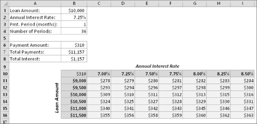
Figure 15.8 Using a two-way data table to display payment amounts for various loan amounts and interest rates.

To create this two-way data table, follow these steps:

1. Enter a formula that returns the results that will be used in the data table. In this example, the formula is in cell B6. The formulas in B7:B8 are not used.

2. Enter various values for the first input in successive columns. In this example, the first input value is interest rate, and the values for various interest rates appear in C10:I10.

3. Enter various values for the second input cell in successive rows, to the left and below the input values for the first input. In this example, the second input value is the loan amount, and the values for various loan amounts are in B11:B16.

4. Create a reference to the formula that will be calculated in the table. This reference goes in the upper-left corner of the data table range. In this example, cell B10 contains the following formula:

=B6

5. Select the rectangular range that contains the entries from the previous steps. In this example, select B10:I16.

6. Choose Data Data Tools What-If Analysis Data Table. Excel displays the Data Table dialog box (refer to Figure 15.7).

7. For the Row Input Cell field, specify the cell reference that corresponds to the first input cell. In this example, the Row Input cell is B2.

8. For the Column Input Cell field, specify the cell reference that corresponds to the second input cell. In this example, the Column Input cell is B1.

9. Click OK. Excel inserts an array formula that uses the TABLE function with two arguments.

After you create the two-way data table, you can change the calculated cell by changing the cell reference in the upper-left cell of the data table. In this example, you can change the formula in cell B10 to =B8 (to display total interest) or =B7 (to display total payments).

Tip

If you create very large data tables, the calculation speed of your workbook may be slowed down. Excel has a special calculation mode for calculation-intensive data tables. To change the calculation mode, choose Formulas Calculation Calculation Options Automatic Except for Data Tables.

Calculating a loan with irregular payments

So far, the loan calculation examples in this chapter have involved loans with regular periodic payments. In some cases, loan payback is irregular. For example, you may loan some money to a friend without a formal agreement as to how he'll pay the money back. You still collect interest on the loan, so you need a way to perform the calculations based on the actual payment dates.

Figure 15.9 shows a worksheet set up to keep track of such a loan. The annual interest rate for the loan is stored in cell B1 (named APR). The original loan amount and loan date are stored in row 5. Notice that the loan amount is entered as a negative value in cell B5. Formulas, beginning in row 6, track the irregular loan payments and perform calculations.

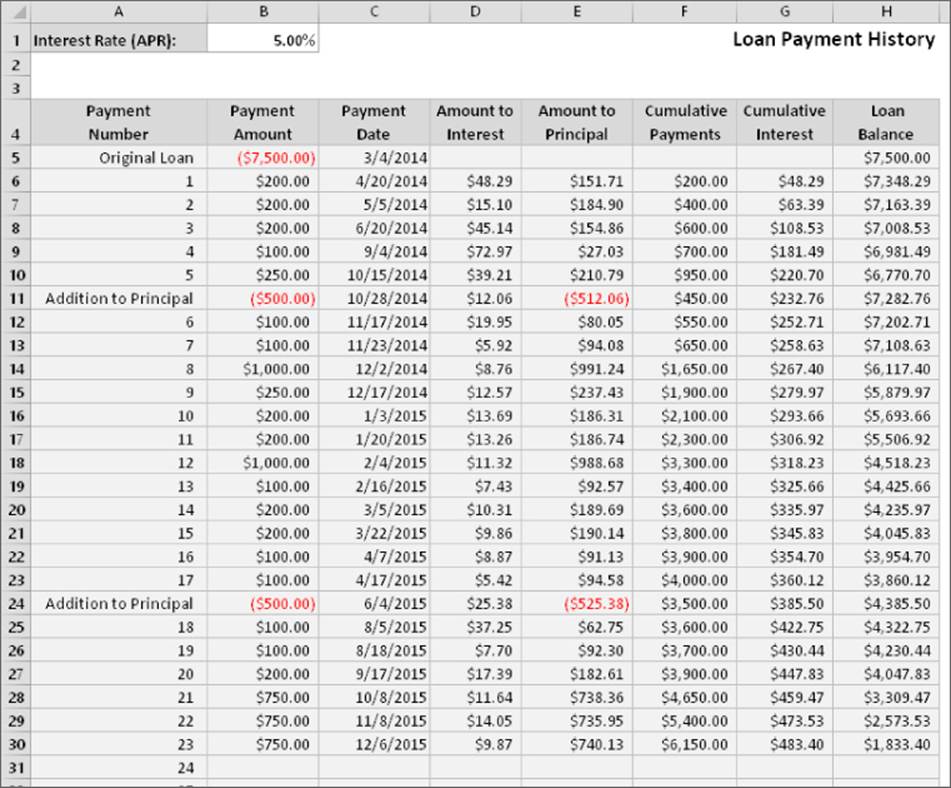
Figure 15.9 This worksheet tracks loan payments that are made on an irregular basis.

Column B stores the payment amount made on the date in column C. Notice that the payments are not made on a regular basis. Also, notice that in two cases (row 11 and row 24), the payment amount is negative. These entries represent additional borrowed money added to the loan balance. Formulas in columns D and E calculate the amount of the payment credited toward interest and principal. Columns F and G keep a running tally of the cumulative payments and interest amounts. Formulas in column H compute the new loan balance after each payment.

Table 15.3 lists and describes the formulas in row 6. Note that each formula uses an IF function to determine whether the payment date in column C is missing. If so, the formula returns an empty string, so no data appears in the cell.

Table 15.3 Formulas to Calculate a Loan with Irregular Payments

This workbook is available on the book's website at www.wiley.com/go/excel2016bible. The filename is irregular payments.xlsx.

Investment Calculations

Investment calculations involve calculating interest on fixed-rate investments, such as bank savings accounts, CDs, and annuities. You can make these interest calculations for investments that consist of a single deposit or multiple deposits.

This book's website at www.wiley.com/go/excel2016bible contains a workbook with all the interest calculation examples in this section. The file is named investment calculations.xlsx.

Future value of a single deposit

Many investments consist of a single deposit that earns interest over the term of the investment. This section describes calculations for simple interest and compound interest.

Calculating simple interest

Simple interest refers to the fact that interest payments are not compounded. The basic formula for computing interest is

Interest=Principal*Rate*Term

For example, suppose that you deposit $1,000 into a bank CD that pays a 3% simple annual interest rate. After one year, the CD matures, and you withdraw your money. The bank adds $30, and you walk away with $1,030. In this case, the interest earned is calculated by multiplying the principal ($1,000) by the interest rate (0.03) by the term (one year).

If the investment term is less than one year, the simple interest rate is adjusted accordingly, based on the term. For example, $1,000 invested in a six-month CD that pays 3% simple annual interest earns $15.00 when the CD matures. In this case, the annual interest rate multiplies by ⁶/₁₂.

Figure 15.10 shows a worksheet set up to make simple interest calculations. The formula in cell B7, shown here, calculates the interest due at the end of the term:

=B3*B4*B5

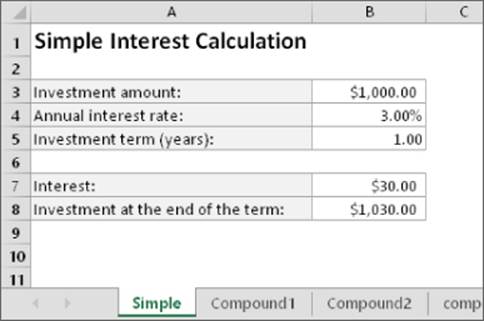
Figure 15.10 This worksheet calculates simple interest payments.

The formula in B8 simply adds the interest to the original investment amount.

Calculating compound interest

Most fixed-term investments pay interest by using some type of compound interest calculation. Compound interest refers to interest credited to the investment balance, and the investment then earns interest on the interest.

For example, suppose that you deposit $1,000 into a bank CD that pays 3% annual interest rate, compounded monthly. Each month, the interest is calculated on the balance, and that amount is credited to your account. The next month's interest calculation will be based on a higher amount because it also includes the previous month's interest payment. One way to calculate the final investment amount involves a series of formulas (see Figure 15.11).

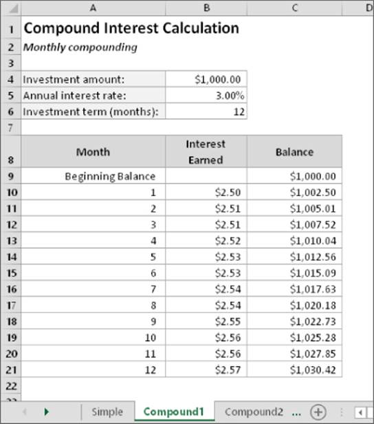
Figure 15.11 Using a series of formulas to calculate compound interest.

Column B contains formulas to calculate the interest for one month. For example, the formula in B10 is

=C9*($B$5*(1/12))

The formulas in column C add the monthly interest amount to the balance. For example, the formula in C10 is

=C9+B10

At the end of the 12-month term, the CD balance is $1,030.42. In other words, monthly compounding results in an additional $0.42 (compared with simple interest).

You can use the FV (future value) function to calculate the final investment amount without using a series of formulas. Figure 15.12 shows a worksheet set up to calculate compound interest. Cell B6 is an input cell that holds the number of compounding periods per year. For monthly compounding, the value in B6 would be 12. For quarterly compounding, the value would be 4. For daily compounding, the value would be 365. Cell B7 holds the term of the investment expressed in years.

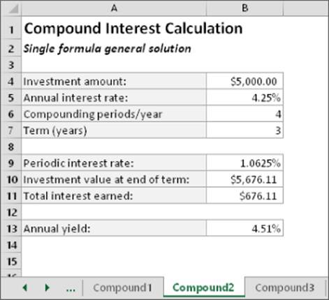
Figure 15.12 Using a single formula to calculate compound interest.

Cell B9 contains the following formula that calculates the periodic interest rate. This value is the interest rate used for each compounding period.

=B5*(1/B6)

The formula in cell B10 uses the FV function to calculate the value of the investment at the end of the term. The formula is

=FV(B9,B6*B7,,-B4)

The first argument for the FV function is the periodic interest rate, which is calculated in cell B9. The second argument represents the total number of compounding periods. The third argument (pmt) is omitted, and the fourth argument is the original investment amount (expressed as a negative value).

The total interest is calculated with a simple formula in cell B11:

=B10-B4

Another formula, in cell B13, calculates the annual yield on the investment:

=(B11/B4)/B7

For example, suppose that you deposit $5,000 into a three-year CD with a 4.25% annual interest rate compounded quarterly. In this case, the investment has four compounding periods per year, so you enter 4 into cell B6. The term is three years, so you enter 3 into cell B7. The formula in B10 returns $5,676.11.

Perhaps you want to see how this rate stacks up against a competitor's account that offers daily compounding. Figure 15.13 shows a calculation with daily compounding, using a $5,000 investment. (Compare this with Figure 15.12.) As you can see, the difference is very small ($679.88 versus $676.11). Over a period of three years, the account with daily compounding earns a total of $3.77 more interest. In terms of annual yield, quarterly compounding earns 4.51%, and daily compounding earns 4.53%.

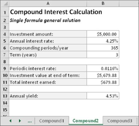
Figure 15.13 Calculating interest by using daily compounding.

Calculating interest with continuous compounding

The term continuous compounding refers to interest that is accumulated continuously. In other words, the investment has an infinite number of compounding periods per year. The following formula calculates the future value of a $5,000 investment at 4.25% compounded continuously for three years:

=5000*EXP(4.25%*3)

The formula returns $5,679.92, which is an additional $0.04 compared with daily compounding.

Note

You can calculate compound interest without using the FV function. The general formula to calculate compound interest is

Principal*(1+Periodic Rate)^Number of Periods

For example, consider a five-year, $5,000 investment that earns an annual interest rate of 4%, compounded monthly. The formula to calculate the future value of this investment is

=5000*(1+4%/12)^(12*5)

The Rule of 72

Need to make an investment decision but don't have a computer handy? You can use the Rule of 72 to determine the number of years required to double your money at a particular interest rate, using annual compounding. Just divide 72 by the interest rate. For example, consider a $10,000 investment at 4% interest. How many years will it take to turn that 10 grand into 20 grand? Take 72, divide it by 4, and you get 18 years. What if you can get a 5% interest rate? If so, you can double your money in a little over 14 years.

How accurate is the Rule of 72? The table that follows shows Rule of 72 estimated years versus the actual years for various interest rates. As you can see, this simple rule is remarkably accurate. However, for interest rates that exceed 30 percent, the accuracy drops off considerably.

The Rule of 72 also works in reverse. For example, if you want to double your money in six years, divide 6 into 72; you'll discover that you need to find an investment that pays an annual interest rate of about 12%. Good luck.

Future value of a series of deposits

Now consider another type of investment, one in which you make a regular series of deposits into an account. This type of investment is known as an annuity.

The worksheet functions discussed in the “Loan Calculations” section earlier in this chapter also apply to annuities, but you need to use the perspective of a lender, not a borrower. A simple example of this type of investment is a holiday club savings program offered by some banking institutions. A fixed amount is deducted from each of your paychecks and deposited into an interest-earning account. At the end of the year, you withdraw the money (with accumulated interest) to use for holiday expenses.

Suppose that you deposit $200 at the beginning of each month (for 12 months) into an account that pays 2.5% annual interest compounded monthly. The following formula calculates the future value of your series of deposits:

=FV(2.5%/12,12,-200,,1)

This formula returns $2,432.75, which represents the total of your deposits ($2,400.00) plus the interest ($32.75). The last argument for the FV function is 1, which means that you make payments at the beginning of the month. Figure 15.14 shows a worksheet set up to calculate annuities. Table 15.4 describes the contents of this sheet.

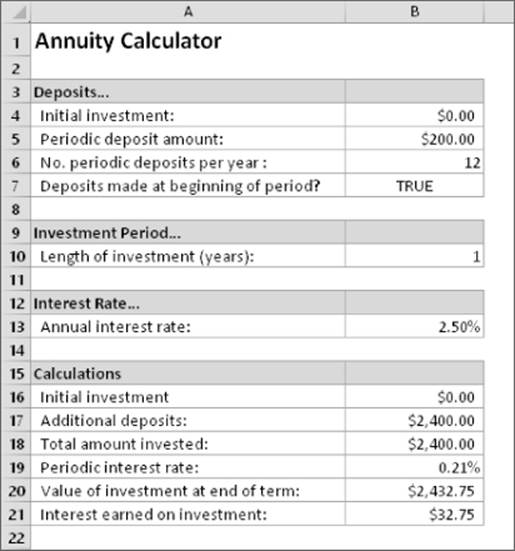
Figure 15.14 This worksheet contains formulas to calculate annuities.

Table 15.4 The Annuity Calculator Worksheet

The workbook shown in Figure 15.14 is available on this book's website at www.wiley.com/go/excel2016bible. The file is named annuity calculator.xlsx.

Depreciation Calculations

Excel offers five functions to calculate depreciation of an asset over time. Depreciating an asset places a value on the asset at a point in time, based on the original value and its useful life. The function that you choose depends on the type of depreciation method you use.

Table 15.5 summarizes the Excel depreciation functions and the arguments used by each. For complete details, consult the Excel online Help system.

Table 15.5 Excel Depreciation Functions

^* Optional

Here are the arguments for the depreciation functions:

· Cost: Original cost of the asset.

· Salvage: Salvage cost of the asset after it has fully depreciated.

· Life: Number of periods over which the asset will depreciate.

· Period: Period in the life for which the calculation is being made.

· Month: Number of months in the first year; if omitted, Excel uses 12.

· Start_Period: Starting period for the depreciation calculation.

· End_Period: Ending period for the depreciation calculation.

· Factor: Rate at which the balance declines; if omitted, it is assumed to be 2 (that is, double-declining).

· No Switch: TRUE or FALSE. Specifies whether to switch to straight-line depreciation when depreciation is greater than the declining balance calculation.

Figure 15.15 shows depreciation calculations using the SLN, DB, DDB, and SYD functions. The asset's original cost, $10,000, is assumed to have a useful life of ten years, with a salvage value of $1,000. The range labeled Depreciation Amount shows the annual depreciation of the asset. The range labeled Value of Asset shows the asset's depreciated value over its life.

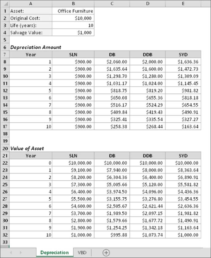
Figure 15.15 A comparison of four depreciation functions.

This workbook is available on this book's website at www.wiley.com/go/excel2016bible. The file is named depreciation calculations.xlsx.

Figure 15.16 shows a chart that graphs the asset's value. As you can see, the SLN function produces a straight line; the other functions produce a curved line because the depreciation is greater in the earlier years of the asset's life.

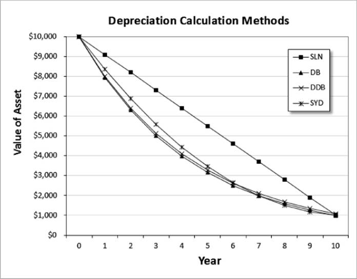
Figure 15.16 This chart shows an asset's value over time, using four depreciation functions.

The VBD function is useful if you need to calculate depreciation for multiple periods (for example, years 2 and 3). Figure 15.17 shows a worksheet set up to calculate depreciation using the VBD function. The formula in cell B11 is

=VDB(B2,B4,B3,B6,B7,B8,B9)

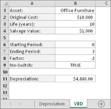
Figure 15.17 Using the VBD function to calculate depreciation for multiple periods.

The formula displays the depreciation for the first three years of an asset (starting period of 0 and ending period of 3).

Financial Forecasting

Forecasting refers to predicting values based on historical values. The values can be financial (for example, sales or income) or any other time-based data (for example, number of employees).

Excel 2016 makes the forecasting process easier than ever.

Note

Excel 2016 includes five new worksheet functions for forecasting. As you see, Excel can insert these functions for you automatically and can even generate a chart.

This workbook is available on this book's website at www.wiley.com/go/excel2016bible. The file is named forecasting example.xlsx.

To create a forecast, start with historical time-based data — for example, monthly sales. Figure 15.18 shows a simple example. Column B contains monthly sales data from 2012 through 2015. I also created a chart, which shows the sales tend to be cyclical, with lower sales during the summer months. The goal is to forecast the monthly sales for the next two years.

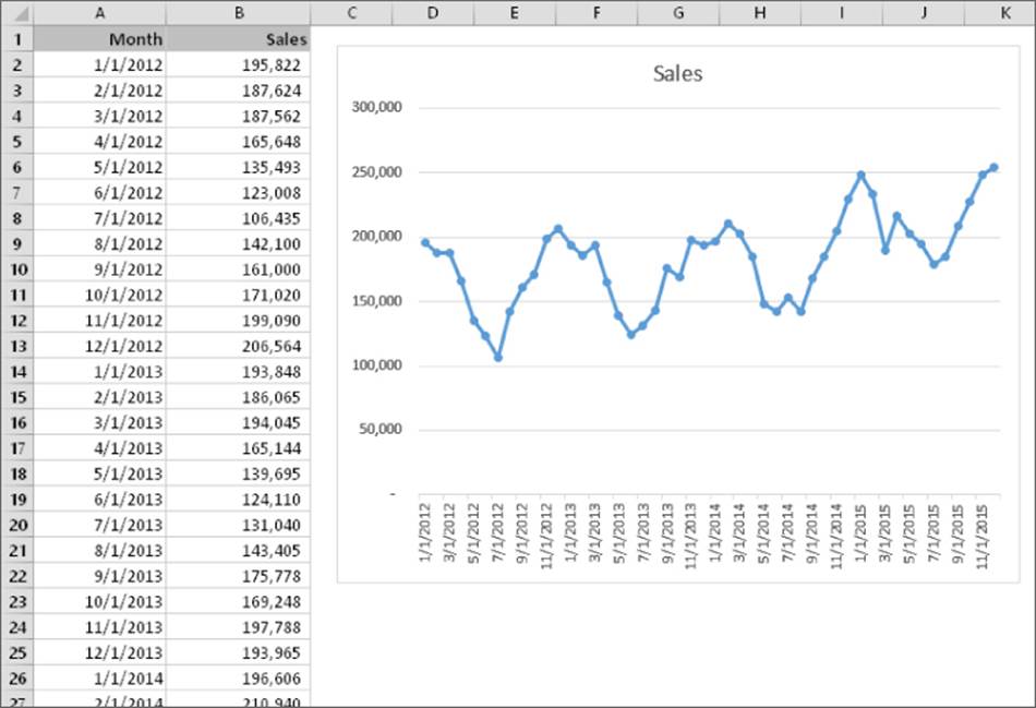
Figure 15.18 Four years of monthly sales data.

Start by selecting the data. For this example, I selected the range A1:B49. Choose Data Forecast Forecast Sheet, and Excel displays the Create Forecast Worksheet dialog box shown in Figure 15.19. (I clicked Options to display additional parameters.) The dialog box shows a chart that displays the historical data, the forecasted data, and the confidence limits for the forecast.

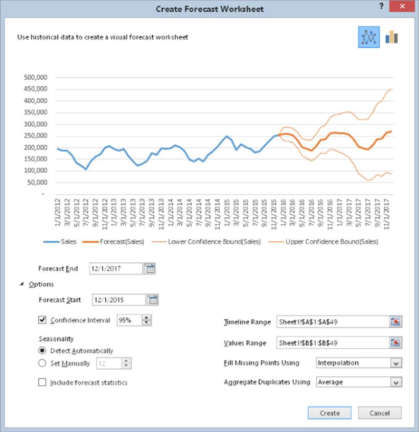
Figure 15.19 The Create Forecast Worksheet dialog box.

The confidence interval (depicted as thinner lines in the chart) determines the “plus or minus” values for the forecast and indicates the degree of confidence in the forecast. A higher confidence interval results in a wider prediction range.

Note that the chart shown in the dialog box adjusts as you change options.

Click Create, and Excel inserts a new worksheet that contains a table and a chart. Figure 15.20 shows part of this table. The table displays the forecasted values, along with the lower and upper confidence intervals. These values are generated using the newFORECAST.ETS and FORECAST.ETS.CONFINT functions. These are fairly complex functions, which explains why Excel does all the work.

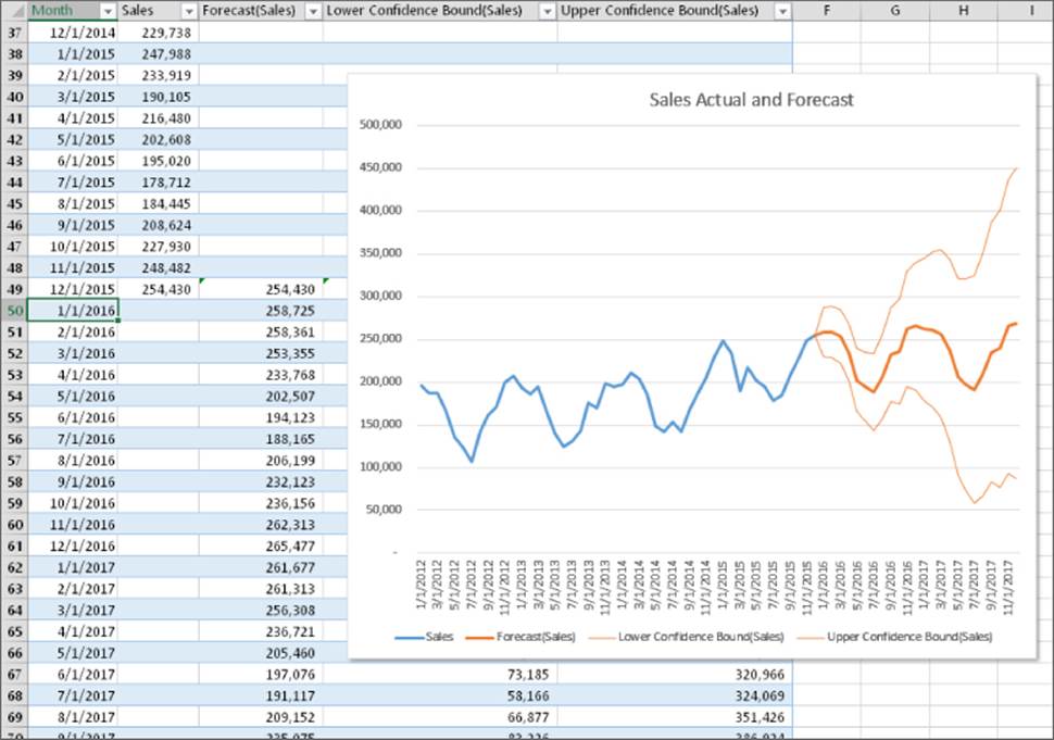
Figure 15.20 The forecast worksheet contains a table and a chart.