Microsoft Excel 2016 BIBLE (2016)

IN THIS CHAPTER

1. Converting between measurement units

2. Solving right triangles

3. Calculating area, surface, circumference, and volume

4. Demonstrating various ways to round numbers

This chapter contains reference information that may be useful to you at some point. Consider it a cheat sheet to help you remember the stuff you may have learned but have long since forgotten.

Unit Conversions

You know the distance from New York to London in miles, but your European office needs the ­number in kilometers. What's the conversion factor?

Excel's CONVERT function can convert between a variety of measurements in the following categories:

· Area

· Distance

· Energy

· Force

· Information

· Magnetism

· Power

· Pressure

· Speed

· Temperature

· Time

· Volume (or liquid measure)

· Weight and mass

Note

Prior to Excel 2007, the CONVERT function required the Analysis ToolPak add-in. Beginning with Excel 2007, this useful function is built in.

The CONVERT function requires three arguments: the value that you want to convert, the from-unit, and the to-unit. For example, if cell A1 contains a distance expressed in miles, use this formula to convert miles to kilometers:

=CONVERT(A1,"mi","km")

The second and third arguments are unit abbreviations, which are listed in the Excel Help system. Some of the abbreviations are commonly used, but others aren't. And, of course, you must use the exact abbreviation. Furthermore, the unit abbreviations are case sensitive, so the following formula returns an error:

=CONVERT(A1,"Mi","km")

The CONVERT function is even more versatile than it seems. When using metric units, you can apply a multiplier. In fact, the first example I presented uses a multiplier. The actual unit abbreviation for the third argument is m for meters. I added the kilo-multiplier (k) to express the result in kilometers.

Sometimes you need to use a bit of creativity. For example, if you need to convert 100 km/hour into miles/sec, the following formula uses the CONVERT function:

=CONVERT(100,"km","mi")/CONVERT(1,"hr","sec")

Note

The CONVERT function was significantly enhanced in Excel 2013 and includes dozens of new units. Therefore, you need to be careful if you use this function in workbooks that will be opened in earlier versions of Excel.

Figure 16.1 shows part of a table that lists all the conversion units supported by the CONVERT function. The table can be sorted and filtered, and it indicates which of the units support the metric prefixes and which were introduced in Excel 2013.

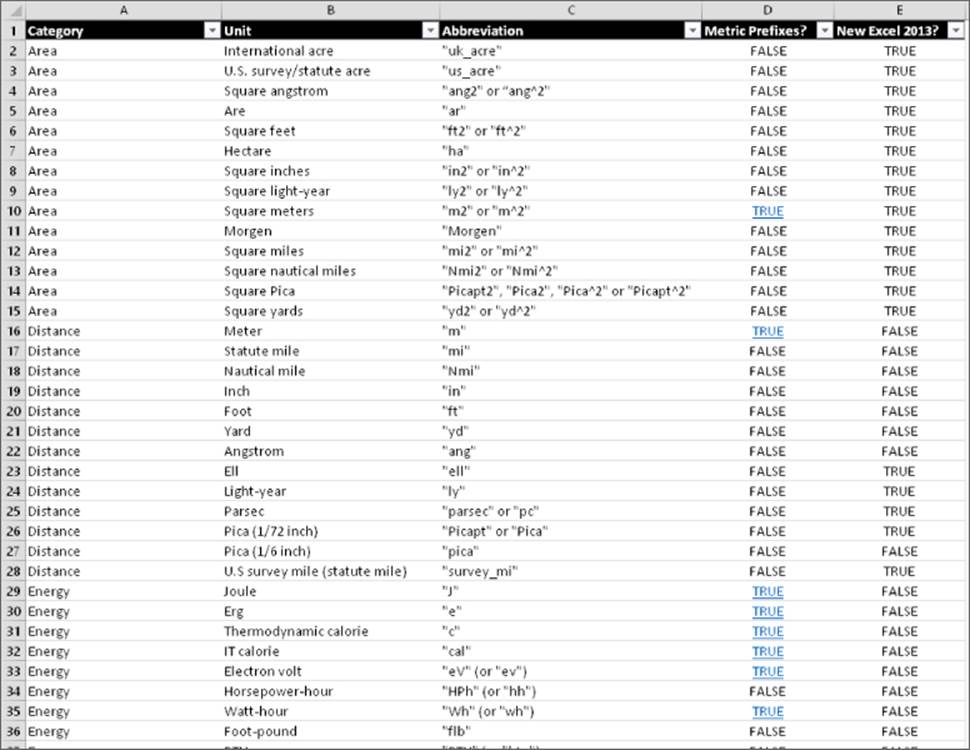
Figure 16.1 A table that lists all the units supported by the CONVERT function.

This workbook is available on this book's website at www.wiley.com/go/excel2016bible. The filename is conversion units table.xlsx.

If you can't find a particular unit that works with the CONVERT function, it's possible that Excel has another function that will do the job. Table 16.1 lists some other functions that convert between measurement units.

Table 16.1 Other Conversion Functions

^* Function introduced in Excel 2013

Solving Right Triangles

A right triangle has six components: three sides and three angles. Figure 16.2 shows a right triangle with its various parts labeled. Angles are labeled A, B, and C; sides are labeled Hypotenuse, Adjacent, and Opposite. Angle C is always 90 degrees (or π/2 radians). If you know any two of these components (excluding angle C, which is always known), you can use formulas to solve for the others.

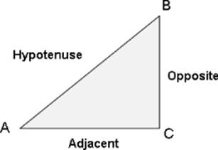
Figure 16.2 A right triangle's components.

The Pythagorean theorem states that Opposite² + Adjacent² = Hypotenuse². Therefore, if you know two sides of a right triangle, you can calculate the remaining side. The formula to calculate a right triangle's opposite side (given the length of the hypotenuse and adjacent side) is as follows:

=SQRT((hypotenuse^2)-(adjacent^2))

The formula to calculate a right triangle's adjacent side (given the length of the hypotenuse and opposite side) is as follows:

=SQRT((hypotenuse^2)-(opposite^2))

The formula to calculate a right triangle's hypotenuse (given the length of the adjacent and opposite sides) is as follows:

=SQRT((opposite^2)+(adjacent^2))

Other useful trigonometric identities are

SIN(A) = opposite/hypotenuse

SIN(B) = adjacent/hypotenuse

COS(A) = adjacent/hypotenuse

COS(B) = opposite/hypotenuse

TAN(A) = opposite/adjacent

TAN(B) = adjacent/opposite

Note

Excel's trigonometric functions assume that the angle arguments are in radians. To convert degrees to radians, use the RADIANS function. To convert radians to degrees, use the DEGREES function.

If you know the opposite and adjacent sides, you can use the following formula to calculate the angle formed by the hypotenuse and adjacent side (angle A):

=ATAN(opposite/adjacent)

The preceding formula returns radians. To convert to degrees, use this formula:

=DEGREES(ATAN(opposite/adjacent))

If you know the opposite and adjacent sides, you can use the following formula to calculate the angle formed by the hypotenuse and the opposite side (angle B):

=PI()/2-ATAN(opposite/adjacent)

The preceding formula returns radians. To convert to degrees, use this formula:

=90-DEGREES(ATAN(opposite/adjacent))

Area, Surface, Circumference, and Volume Calculations

This section contains formulas for calculating the area, surface, circumference, and volume for common two- and three-dimensional shapes.

Calculating the area and perimeter of a square

To calculate the area of a square, square the length of one side. The following formula calculates the area of a square for a cell named side:

=side^2

To calculate the perimeter of a square, multiply one side by 4. The following formula uses a cell named side to calculate the perimeter of a square:

=side*4

Calculating the area and perimeter of a rectangle

To calculate the area of a rectangle, multiply its height by its base. The following formula returns the area of a rectangle, using cells named height and base:

=height*base

To calculate the perimeter of a rectangle, multiply the height by 2 and then add it to the width multiplied by 2. The following formula returns the perimeter of a rectangle, using cells named height and width:

=(height*2)+(width*2)

Calculating the area and perimeter of a circle

To calculate the area of a circle, multiply the square of the radius by π. The following formula returns the area of a circle. It assumes that a cell named radius contains the circle's radius:

=pi()*(radius^2)

The radius of a circle is equal to one-half of the diameter.

To calculate the circumference of a circle, multiply the diameter of the circle by π. The following formula calculates the circumference of a circle using a cell named diameter:

=diameter*pi()

The diameter of a circle is the radius times 2.

Calculating the area of a trapezoid

To calculate the area of a trapezoid, add the two parallel sides, multiply by the height, and then divide by 2. The following formula calculates the area of a trapezoid using cells named parallel_side_1, parallel_side_2, and height:

=((parallel_side_1+parallel_side_2)*height)/2

Calculating the area of a triangle

To calculate the area of a triangle, multiply the base by the height and then divide by 2. The following formula calculates the area of a triangle using cells named base and height:

=(base*height)/2

Calculating the surface and volume of a sphere

To calculate the surface of a sphere, multiply the square of the radius by π and then multiply by 4. The following formula returns the surface of a sphere, the radius of which is in a cell named radius:

=pi()*(radius^2)*4

To calculate the volume of a sphere, multiply the cube of the radius by 4 times π and then divide by 3. The following formula calculates the volume of a sphere. The cell named radius contains the sphere's radius:

=((radius^3)*(4*pi()))/3

Calculating the surface and volume of a cube

To calculate the surface area of a cube, square one side and multiply by 6. The following formula calculates the surface of a cube using a cell named side, which contains the length of a side of the cube:

=(side^2)*6

To calculate the volume of a cube, raise the length of one side to the third power. The ­following formula returns the volume of a cube using a cell named side:

=side^3

Calculating the surface and volume of a rectangular solid

The following formula calculates the surface of a rectangular solid using cells named height, width, and length:

=(length*height*2)+(length*width*2)+(width*height*2)

To calculate the volume of a rectangular solid, multiply the height by the width by the length:

=height*width*length

Calculating the surface and volume of a cone

The following formula calculates the surface of a cone (including the surface of the base). This formula uses cells named radius and height:

=pi()*radius*(SQRT(height^2+radius^2)+radius))

To calculate the volume of a cone, multiply the square of the radius of the base by π, multiply by the height, and then divide by 3. The following formula returns the volume of a cone using cells named radius and height:

=(pi()*(radius^2)*height)/3

Calculating the volume of a cylinder

To calculate the volume of a cylinder, multiply the square of the radius of the base by π and then multiply by the height. The following formula calculates the volume of a cylinder using cells named radius and height:

=(pi()*(radius^2)*height)

Calculating the volume of a pyramid

Calculate the area of the base, multiply by the height, and then divide by 3. This formula calculates the volume of a pyramid. It assumes cells named width (the width of the base), length (the length of the base), and height (the height of the pyramid):

=(width*length*height)/3

Rounding Numbers

Excel provides quite a few functions that round values in various ways. Table 16.2 summarizes these functions.

Table 16.2 Excel Rounding Functions

^* Introduced in Excel 2010

Caution

It's important to understand the difference between rounding a value and formatting a value. When you format a number to display a specific number of decimal places, formulas that refer to that number use the actual value, which may differ from the displayed value. When you round a number, formulas that refer to that value use the rounded number.

The following sections provide examples of formulas that use various types of rounding.

Basic rounding formulas

The ROUND function is useful for basic rounding to a specified number of digits. You specify the number of digits in the second argument for the ROUND function. For example, the ­formula that follows returns 123.40. (The value is rounded to one decimal place.)

=ROUND(123.37,1)

If the second argument for the ROUND function is zero, the value is rounded to the nearest integer. The formula that follows, for example, returns 123.00:

=ROUND(123.37,0)

The second argument for the ROUND function can also be negative. In such a case, the number is rounded to the left of the decimal point. The following formula, for example, returns 120.00:

=ROUND(123.37,–1)

The ROUND function rounds either up or down. But how does it handle a number such as 12.5, rounded to no decimal places? You'll find that the ROUND function rounds such numbers away from zero. The formula that follows, for instance, returns 13.0:

=ROUND(12.5,0)

The next formula returns –13.00. (The rounding occurs away from zero.)

=ROUND(–12.5,0)

To force rounding to occur in a particular direction, use the ROUNDUP or ROUNDDOWN functions. The following formula, for example, returns 12.0. The value rounds down:

=ROUNDDOWN(12.5,0)

The formula that follows returns 13.0. The value rounds up to the nearest whole value:

=ROUNDUP(12.43,0)

Rounding to the nearest multiple

The MROUND function is useful for rounding values to the nearest multiple. For example, you can use this function to round a number to the nearest 5. The following formula returns 135:

=MROUND(133,5)

Rounding currency values

Often, you need to round currency values. For example, you may need to round a dollar amount to the nearest penny. A calculated price may be something like $45.78923. In such a case, you'll want to round the calculated price to the nearest penny. This may sound simple, but there are actually three ways to round such a value:

· Round it up to the nearest penny.

· Round it down to the nearest penny.

· Round it to the nearest penny. (The rounding may be up or down.)

The following formula assumes that a dollar-and-cents value is in cell A1. The formula rounds the value to the nearest penny. For example, if cell A1 contains $12.421, the formula returns $12.42:

=ROUND(A1,2)

If you need to round the value up to the nearest penny, use the CEILING function. The following formula rounds the value in cell A1 up to the nearest penny. For example, if cell A1 contains $12.421, the formula returns $12.43:

=CEILING(A1,0.01)

To round a dollar value down, use the FLOOR function. The following formula, for example, rounds the dollar value in cell A1 down to the nearest penny. If cell A1 contains $12.421, the formula returns $12.42:

=FLOOR(A1,0.01)

To round a dollar value up to the nearest nickel, use this formula:

=CEILING(A1,0.05)

You've probably noticed that many retail prices end in $0.99. If you have an even dollar price and you want it to end in $0.99, just subtract $0.01 from the price. Some higher-ticket items are always priced to end with $9.99. To round a price to the nearest $9.99, first round it to the nearest $10.00 and then subtract a penny. If cell A1 contains a price, use a formula like this to convert it to a price that ends in $9.99:

=ROUND(A1/10,0)*10–0.01

For example, if cell A1 contains $345.78, the formula returns $349.99.

A simpler approach uses the MROUND function:

=MROUND(A1,10)–0.01

Working with fractional dollars

The DOLLARFR and DOLLARDE functions are useful when you're working with fractional dollar value, as in stock market quotes.

Consider the value $9.25. You can express the decimal part as a fractional value ($91/4, $92/8, $94/16, and so on). The DOLLARFR function takes two arguments: the dollar amount and the denominator for the fractional part. The following formula, for example, returns 9.1. (The .1 decimal represents 1/4.)

=DOLLARFR(9.25,4)

Caution

In most situations, you won't use the value returned by the DOLLARFR function in other calculations. In the preceding example, the result of the function will be interpreted as 9.1, not 9.25. To perform calculations on such a value, you need to convert it back to a decimal value by using the DOLLARDE function.

The DOLLARDE function converts a dollar value expressed as a fraction to a decimal amount. It also uses a second argument to specify the denominator of the fractional part. The following formula, for example, returns 9.25:

=DOLLARDE(9.1,4)

Tip

The DOLLARDE and DOLLARFR functions aren't limited to dollar values. For example, you can use these functions to work with feet and inches. You might have a value that represents 81/2 feet. Use the following formula to express this value in terms of feet and inches. The formula returns 8.06 (which represents 8 feet, 6 inches).

=DOLLARFR(8.5,12)

Another example is baseball statistics. A pitcher may work 62/3 innings, which is usually represented as 6.2. The following formula displays 6.2:

=DOLLARFR(6+2/3,3)

Using the INT and TRUNC functions

On the surface, the INT and TRUNC functions seem similar. Both convert a value to an integer. The TRUNC function simply removes the fractional part of a number. The INT function rounds a number down to the nearest integer, based on the value of the fractional part of the number.

In practice, INT and TRUNC return different results only when using negative numbers. For example, the following formula returns –14.0:

=TRUNC(–14.2)

The next formula returns –15.0 because –14.2 is rounded down to the next lower integer:

=INT(–14.2)

The TRUNC function takes an additional (optional) argument that's useful for truncating decimal values. For example, the formula that follows returns 54.33 (the value truncated to two decimal places):

=TRUNC(54.3333333,2)

Rounding to an even or odd integer

The ODD and EVEN functions are provided when you need to round a number up to the nearest odd or even integer. These functions take a single argument and return an integer value. The EVEN function rounds its argument up to the nearest even integer. The ODDfunction rounds its argument up to the nearest odd integer. Table 16.3 shows some examples of these functions.

Table 16.3 Results Using the EVEN and ODD Functions

Rounding to n significant digits

In some cases, you may need to round a value to a particular number of significant digits. For example, you might want to express the value 1,432,187 in terms of two significant digits (that is, as 1,400,000). The value 9,187,877 expressed in terms of three significant digits is 9,180,000.

If the value is a positive number with no decimal places, the following formula does the job. This formula rounds the number in cell A1 to two significant digits. To round to a different number of significant digits, replace the 2 in this formula with a different number.

=ROUNDDOWN(A1,2–LEN(A1))

For nonintegers and negative numbers, the solution gets a bit trickier. The formula that follows provides a more general solution that rounds the value in cell A1 to the number of significant digits specified in cell A2. This formula works for positive and negative integers and nonintegers.

=ROUND(A1,A2–1–INT(LOG10(ABS(A1))))

For example, if cell A1 contains 1.27845 and cell A2 contains 3, the formula returns 1.28000 (the value, rounded to three significant digits).