Microsoft Excel 2016 BIBLE (2016)
Part II
Working with Formulas and Functions
Chapter 17
Introducing Array Formulas
IN THIS CHAPTER
1. Defining arrays and array formulas
2. Comparing one-dimensional and two-dimensional arrays
3. Working with array constants
4. Working with array formulas
5. Looking at examples of multicell array formulas
6. Looking at examples of single-cell array formulas
One of Excel's most interesting (and most powerful) features is its ability to work with arrays in formulas. When you understand this concept, you'll be able to create elegant formulas that appear to perform spreadsheet magic.
This chapter introduces the concept of arrays and is required reading for anyone who wants to become a master of Excel formulas. Chapter 18, “Performing Magic with Array Formulas,” continues with lots of useful examples.
 Most of the examples in this chapter are available on this book's website at www.wiley.com/go/excel2016bible. The filename is array examples.xlsx.
Understanding Array Formulas
If you do any computer programming, you've probably been exposed to the concept of an array. An array is a collection of items operated on collectively or individually. In Excel, an array can be one dimensional or two dimensional. These dimensions correspond to rows and columns. For example, a one-dimensional array can be stored in a range that consists of one row (a horizontal array) or one column (a vertical array). A two-dimensional array can be stored in a rectangular range of cells. Excel doesn't support three-dimensional arrays (but its VBA programming language does).
As you'll see, arrays don't have to be stored in cells. You can also work with arrays that exist only in Excel's memory. Then you can use an array formula to manipulate this information and return a result. Excel supports two types of array formulas:
· Single-cell array formulas: Work with arrays stored in ranges or in memory and produce a result displayed in a single cell.
· Multicell array formulas: Work with arrays stored in ranges or in memory and produce an array as a result. Because a cell can hold only one value, a multicell array formula is entered into a range of cells.
This section presents two array formula examples: one that occupies multiple cells and another that occupies only one cell.
A multicell array formula
Figure 17.1 shows a simple worksheet set up to calculate product sales. Normally, you'd calculate the value in column D (total sales per product) with a formula such as the one that follows, and then you'd copy this formula down the column.
=B2*C2
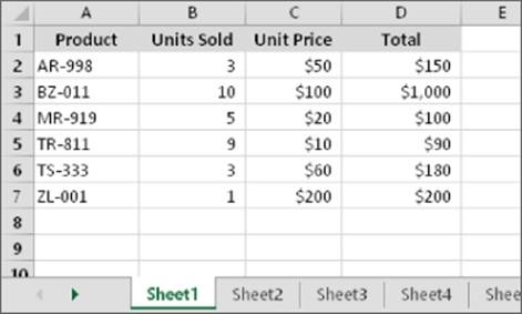
Figure 17.1 Column D contains formulas to calculate the total for each product.
After you copy the formula, the worksheet contains six formulas in column D.
An alternative method uses a single formula (a multicell array formula) to calculate all six values in D2:D7. This single formula occupies six cells and returns an array of six values.
To create a multicell array formula to perform the calculations, follow these steps:
1. Select a range to hold the results. In this case, the range is D2:D7. Because you can't display more than one value in a single cell, six cells are required to display the resulting array — so you select six cells to make this array work.
2. Type the following formula:
=B2:B7*C2:C7
3. Press Ctrl+Shift+Enter to enter the formula. Normally, you press Enter to enter a formula. Because this is an array formula, however, press Ctrl+Shift+Enter.
Caution
You can't insert a multicell array formula into a range that has been designated a table (by choosing Insert ![]() Tables
Tables ![]() Table). In addition, you can't convert a range that contains a multicell array formula to a table.
Table). In addition, you can't convert a range that contains a multicell array formula to a table.
The formula is entered into all six selected cells. If you examine the Formula bar, you see the following:
{=B2:B7*C2:C7}
Excel places curly brackets around the formula to indicate that it's an array formula.
This formula performs its calculations and returns a six-item array. The array formula actually works with two other arrays, both of which happen to be stored in ranges. The values for the first array are stored in B2:B7, and the values for the second array are stored in C2:C7.
This multicell array formula returns the same values as these six normal formulas entered into individual cells in D2:D7:
=B2*C2
=B3*C3
=B4*C4
=B5*C5
=B6*C6
=B7*C7
Using a multicell array formula rather than individual formulas does offer a few advantages:
· It's a good way to ensure that all formulas in a range are identical.
· Using a multicell array formula makes it less likely that you'll overwrite a formula accidentally. You can't change or delete just one cell in a multicell array formula. Excel displays an error message if you attempt to do so.
· Using a multicell array formula will almost certainly prevent novices from tampering with your formulas.
Using a multicell array formula as described in the preceding list also has some potential disadvantages:
· Inserting a new row into the range is impossible. But in some cases, the inability to insert a row is a positive feature. For example, you might not want users to add rows because it would affect other parts of the worksheet.
· If you add new data to the bottom of the range, you need to modify the array formula to accommodate the new data.
A single-cell array formula
Now it's time to take a look at a single-cell array formula. Check out Figure 17.2, which is similar to Figure 17.1. Notice, however, that the formulas in column D have been deleted. The goal is to calculate the sum of the total product sales without using the individual calculations that were in column D.
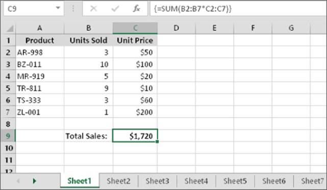
Figure 17.2 The array formula in cell C9 calculates the total sales without using intermediate formulas.
The following array formula is in cell C9:
{=SUM(B2:B7*C2:C7)}
When you enter this formula, make sure that you press Ctrl+Shift+Enter (and don't type the curly brackets because Excel automatically adds them for you).
This formula works with two arrays, both of which are stored in cells. The first array is stored in B2:B7, and the second array is stored in C2:C7. The formula multiplies the corresponding values in these two arrays and creates a new array (which exists only in memory). The new array consists of six values, which can be represented like this. (The reason for using semicolons is explained a bit later.)
{150;1000;100;90;180;200}
The SUM function then operates on this new array and returns the sum of its values.
Note
In this case, you can use the SUMPRODUCT function to obtain the same result without using an array formula:
=SUMPRODUCT(B2:B7,C2:C7)
As you see, however, array formulas allow many other types of calculations that are otherwise not possible.
Creating an Array Constant
The examples in the preceding section used arrays stored in worksheet ranges. The examples in this section demonstrate an important concept: an array doesn't have to be stored in a range of cells. This type of array, which is stored in memory, is referred to as anarray constant.
To create an array constant, list its items and surround them with curly brackets. Here's an example of a five-item horizontal array constant:
{1,0,1,0,1}
The following formula uses the SUM function, with the preceding array constant as its argument. The formula returns the sum of the values in the array (which is 3):
=SUM({1,0,1,0,1})
Notice that this formula uses an array, but the formula itself isn't an array formula. Therefore, you don't press Ctrl+Shift+Enter to enter the formula — although entering it as an array formula will still produce the same result.
Note
When you specify an array directly (as shown previously), you must provide the curly brackets around the array elements. When you enter an array formula, on the other hand, you do not supply the curly brackets.
At this point, you probably don't see any advantage to using an array constant. The following formula, for example, returns the same result as the previous formula. The advantages, however, will become apparent:
=SUM(1,0,1,0,1)
Here's a formula that uses two array constants:
=SUM({1,2,3,4}*{5,6,7,8})
The formula creates a new array (in memory) that consists of the product of the corresponding elements in the two arrays. The new array is
{5,12,21,32}
This new array is then used as an argument for the SUM function, which returns the result (70). The formula is equivalent to the following formula, which doesn't use arrays:
=SUM(1*5,2*6,3*7,4*8)
Alternatively, you can use the SUMPRODUCT function. The formula that follows is not an array formula, but it uses two array constants as its arguments:
=SUMPRODUCT({1,2,3,4},{5,6,7,8})
A formula can work with both an array constant and an array stored in a range. The following formula, for example, returns the sum of the values in A1:D1, each multiplied by the corresponding element in the array constant:
=SUM((A1:D1*{1,2,3,4}))
This formula is equivalent to
=SUM(A1*1,B1*2,C1*3,D1*4)
An array constant can contain numbers, text, logical values (TRUE or FALSE), and even error values, such as #N/A. Numbers can be in integer, decimal, or scientific format. You must enclose text in double quotation marks. You can use different types of values in the same array constant, as in this example:
{1,2,3,TRUE,FALSE,TRUE,"Moe","Larry","Curly"}
An array constant can't contain formulas, functions, or other arrays. Numeric values can't contain dollar signs, commas, parentheses, or percent signs. For example, the following is an invalid array constant:
{SQRT(32),$56.32,12.5%}
Understanding the Dimensions of an Array
As stated previously, an array can be one dimensional or two dimensional. A one-dimensional array's orientation can be horizontal (corresponding to a single row) or vertical (corresponding to a single column).
One-dimensional horizontal arrays
Each element in a one-dimensional horizontal array is separated by a comma, and the array can be displayed in a row of cells. If you use a non-English language version of Excel, your list separator character may be a semicolon.
The following example is a one-dimensional horizontal array constant:
{1,2,3,4,5}
Displaying this array in a range requires five consecutive cells in a row. To enter this array into a range, select a range of cells that consists of one row and five columns. Then enter the following formula and press Ctrl+Shift+Enter:
={1,2,3,4,5}
Note
If you enter this array into a horizontal range that consists of more than five cells, the extra cells will contain #N/A (which denotes unavailable values). If you enter this array into a vertical range of cells, only the first item (1) will appear in each cell.
The following example is another horizontal array; it has seven elements and is made up of text strings:
{"Sun","Mon","Tue","Wed","Thu","Fri","Sat"}
To enter this array, select seven cells in a row and type the following (and then press Ctrl+Shift+Enter):
={"Sun","Mon","Tue","Wed","Thu","Fri","Sat"}
One-dimensional vertical arrays
The elements in a one-dimensional vertical array are separated by semicolons, and the array can be displayed in a column of cells. The following is a six-element vertical array constant:
{10;20;30;40;50;60}
Displaying this array in a range requires six cells in a column. To enter this array into a range, select a range of cells that consists of six rows and one column. Then enter the following formula, followed by Ctrl+Shift+Enter:
={10;20;30;40;50;60}
The following is another example of a vertical array; this one has four elements:
{"Widgets";"Sprockets";"Doodads";"Thingamajigs"}
Two-dimensional arrays
A two-dimensional array uses commas to separate its horizontal elements and semicolons to separate its vertical elements. If you use a non-English language version of Excel, the item-separator character may be a semicolon (for horizontal elements) and a backslash (for vertical elements). If you are not sure, open the example file for this chapter and examine a two-dimensional array. The item-separator characters are translated automatically to your language version.
The following example shows a 3 × 4 array constant:
{1,2,3,4;5,6,7,8;9,10,11,12}
Displaying this array in a range requires 12 cells. To enter this array into a range, select a range of cells that consists of three rows and four columns. Then type the following formula, and press Ctrl+Shift+Enter:
={1,2,3,4;5,6,7,8;9,10,11,12}
Figure 17.3 shows how this array appears when entered into a range (in this case, B3:E5).
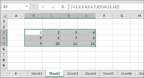
Figure 17.3 A 3 × 4 array entered into a range of cells.
If you enter an array into a range that has more cells than array elements, Excel displays #N/A in the extra cells. Figure 17.4 shows a 3 × 4 array entered into a 10 × 5 cell range.
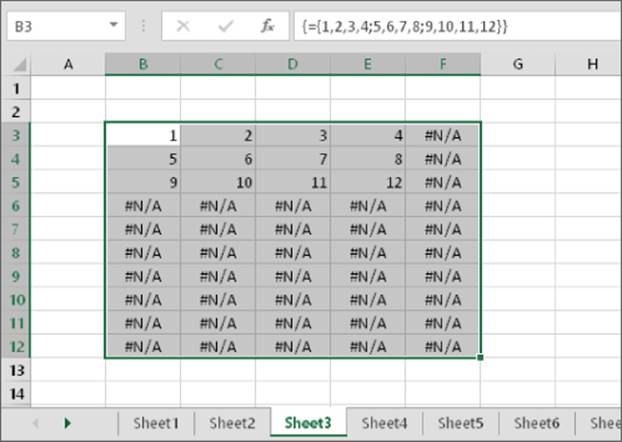
Figure 17.4 A 3 × 4 array entered into a 10 × 5 cell range.
Each row of a two-dimensional array must contain the same number of items. The array that follows, for example, isn't valid, because the third row contains only three items:
{1,2,3,4;5,6,7,8;9,10,11}
Excel doesn't allow you to enter a formula that contains an invalid array.
Naming Array Constants
You can create an array constant, give it a name, and then use this named array in a formula. Technically, a named array is a named formula.
Chapter 4, “Working with Cells and Ranges,” and Chapter 10, “Introducing Formulas and Functions,”cover the topic of names and named formulas.
Figure 17.5 shows a named array being created from the New Name dialog box. (Access this dialog box by choosing Formulas ![]() Defined Names
Defined Names ![]() Define Name.) The name of the array is DayNames, and it refers to the following array constant:
Define Name.) The name of the array is DayNames, and it refers to the following array constant:
{"Sun","Mon","Tue","Wed","Thu","Fri","Sat"}
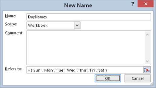
Figure 17.5 Creating a named array constant.
Notice that, in the New Name dialog box, the array is defined (in the Refers To field) using a leading equal sign (=). Without this equal sign, the array is interpreted as a text string rather than an array. Also, you must type the curly brackets when defining a named array constant; Excel doesn't enter them for you.
After creating this named array, you can use it in a formula. Figure 17.6 shows a worksheet that contains a multicell array formula entered into the range B2:H2. The formula is
{=DayNames}
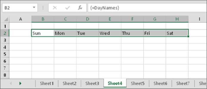
Figure 17.6 Using a named array constant in an array formula.
To enter this formula, select seven cells in a row, type =DayNames, and press Ctrl+Shift+Enter.
Because commas separate the array elements, the array has a horizontal orientation. Use semicolons to create a vertical array. Or you can use the Excel TRANSPOSE function to insert a horizontal array into a vertical range of cells. (See “Transposing an array,” later in this chapter.) The following array formula, which is entered into a seven-cell vertical range, uses the TRANSPOSE function:
{=TRANSPOSE(DayNames)}
You also can access individual elements from the array by using the Excel INDEX function. The following formula, for example, returns Wed, the fourth item in the DayNames array:
=INDEX(DayNames,4)
Working with Array Formulas
This section deals with the mechanics of selecting cells that contain arrays and entering and editing array formulas. These procedures differ a bit from working with ordinary ranges and formulas.
Entering an array formula
When you enter an array formula into a cell or range, you must follow a special procedure so Excel knows that you want an array formula rather than a normal formula. You enter a normal formula into a cell by pressing Enter. You enter an array formula into one or more cells by pressing Ctrl+Shift+Enter.
Don't enter the curly brackets when you create an array formula; Excel inserts them for you. If the result of an array formula consists of more than one value, you must select all the cells in the results range before you enter the formula. If you fail to do so, only the first element of the result is returned.
Selecting an array formula range
You can manually select the cells that contain a multicell array formula by using the normal cell selection procedures. Or you can use either of the following methods:
· Activate any cell in the array formula range. Choose Home ![]() Editing
Editing ![]() Find & Select
Find & Select ![]() Go To, or just press F5. The Go To dialog box appears. In the Go To dialog box, click the Special button and then choose the Current Array option. Click OK to close the dialog box.
Go To, or just press F5. The Go To dialog box appears. In the Go To dialog box, click the Special button and then choose the Current Array option. Click OK to close the dialog box.
· Activate any cell in the array formula range and press Ctrl+/ (forward slash) to select the cells that make up the array.
Editing an array formula
If an array formula occupies multiple cells, you must edit the entire range as though it were a single cell. The key point to remember is that you can't change just one element of a multicell array formula. If you attempt to do so, Excel displays the message shown inFigure 17.7.
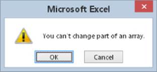
Figure 17.7 Excel's warning message reminds you that you can't edit just one cell of a multicell array formula.
To edit an array formula, select all the cells in the array range and activate the Formula bar as usual. (Click it or press F2.) Excel removes the curly brackets from the formula while you edit it. Edit the formula and then press Ctrl+Shift+Enter to enter the changes. All the cells in the array now reflect your editing changes (and the curly brackets reappear).
The following rules apply to multicell array formulas. If you try to do any of these things, Excel lets you know about it:
· You can't change the contents of any individual cell that makes up an array formula.
· You can't move cells that make up part of an array formula (but you can move an entire array formula).
· You can't delete cells that form part of an array formula (but you can delete an entire array).
· You can't insert new cells into an array range. This rule includes inserting rows or columns that would add new cells to an array range.
· You can't use multicell array formulas inside of a table that was created by choosing Insert ![]() Tables
Tables ![]() Table. Similarly, you can't convert a range to a table if the range contains a multicell array formula.
Table. Similarly, you can't convert a range to a table if the range contains a multicell array formula.
Caution
If you accidentally press Ctrl+Enter (instead of Ctrl+Shift+Enter) after editing an array formula, the formula will be entered into each selected cell, but it will no longer be an array formula. And it will probably return an incorrect result. Just reselect the cells, press F2, and then press Ctrl+Shift+Enter.
Although you can't change any individual cell that makes up a multicell array formula, you can apply formatting to the entire array or to only parts of it.
Expanding or contracting a multicell array formula
Often, you may need to expand a multicell array formula (to include more cells) or contract it (to include fewer cells). Doing so requires these steps:
1. Select the entire range that contains the array formula.
2. Press F2 to enter Edit mode.
3. Press Ctrl+Enter. This step enters an identical (nonarray) formula into each selected cell.
4. Change your range selection to include additional or fewer cells, but make sure the active cell is a cell that's part of the original array.
5. Press F2 to re-enter Edit mode.
6. Press Ctrl+Shift+Enter.
Array Formulas: The Downside
If you've followed along in this chapter, you probably understand some of the advantages of using array formulas. The main advantage, of course, is that an array formula enables you to perform otherwise impossible calculations. As you gain more experience with arrays, however, you undoubtedly will also discover some disadvantages.
Array formulas are one of the least understood features of Excel. Consequently, if you plan to share a workbook with someone who may need to make modifications, you should probably avoid using array formulas. Encountering an array formula when you don't know what it is can be confusing.
You can easily forget to enter an array formula by pressing Ctrl+Shift+Enter. (Also, if you edit an existing array, you must remember to use this key combination to complete the edits.) Except for logical errors, this is probably the most common problem that users have with array formulas. If you press Enter by mistake after editing an array formula, just press F2 to get back into Edit mode and then press Ctrl+Shift+Enter.
Another potential problem with array formulas is that they can sometimes slow your worksheet's recalculations, especially if you use very large arrays. On a faster system, this delay in speed may not be a problem. But, conversely, using an array formula is almost always faster than using a custom VBA function. See Chapter 40, “Creating Custom Worksheet Functions,” for more information about creating custom VBA functions.
Using Multicell Array Formulas
This section contains examples that demonstrate additional features of multicell array formulas (array formulas that are entered into a range of cells). These features include creating arrays from values, performing operations, using functions, transposing arrays, and generating consecutive integers.
Creating an array from values in a range
The following array formula creates an array from a range of cells. Figure 17.8 shows a workbook with some data entered into A1:C4. The range D8:F11 contains a single array formula:
{=A1:C4}
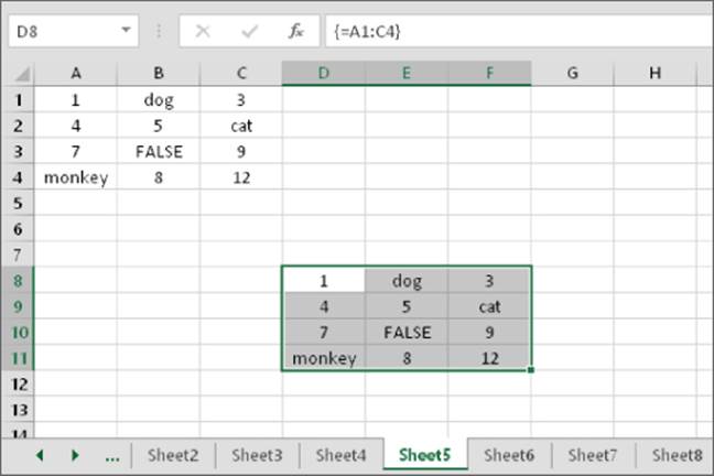
Figure 17.8 Creating an array from a range.
The array in D8:F11 is linked to the range A1:C4. Change any value in A1:C4, and the corresponding cell in D8:F11 reflects that change. It's a one-way link, of course. You can't change a value in D8:F11.
Creating an array constant from values in a range
In the preceding example, the array formula in D8:F11 essentially created a link to the cells in A1:C4. It's possible to sever this link and create an array constant made up of the values in A1:C4:
1. Select the cells that contain the array formula (the range D8:F11, in this example).
2. Press F2 to edit the array formula.
3. Press F9 to convert the cell references to values.
4. Press Ctrl+Shift+Enter to re-enter the array formula (which now uses an array constant).
The array constant is
{1,"dog",3;4,5,"cat";7,False,9;"monkey",8,12}
Figure 17.9 shows how this looks in the Formula bar.
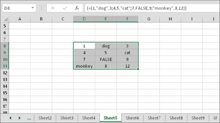
Figure 17.9 After you press F9, the Formula bar displays the array constant.
Performing operations on an array
So far, most of the examples in this chapter simply entered arrays into ranges. The following array formula creates a rectangular array and multiplies each array element by 2:
{={1,2,3,4;5,6,7,8;9,10,11,12}*2}
Figure 17.10 shows the result when you enter this formula into a range:
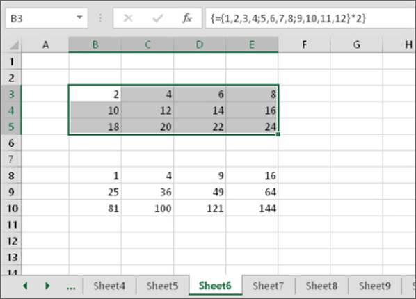
Figure 17.10 Performing a mathematical operation on an array.
The following array formula multiplies each array element by itself:
{={1,2,3,4;5,6,7,8;9,10,11,12}*{1,2,3,4;5,6,7,8;9,10,11,12}}
The following array formula is a simpler way of obtaining the same result. Figure 17.11 shows the result when you enter this formula into a range:
{={1,2,3,4;5,6,7,8;9,10,11,12}^2}
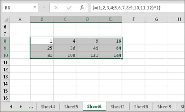
Figure 17.11 Multiplying each array element by itself.
If the array is stored in a range (such as B8:E10), the array formula returns the square of each value in the range, as follows:
{=B8:E10^2}
Using functions with an array
As you may expect, you can also use worksheet functions with an array. The following array formula, which you can enter into a ten-cell vertical range, calculates the square root of each array element in the array constant:
{=SQRT({1;2;3;4;5;6;7;8;9;10})}
If the array is stored in a range, a multicell array formula such as the one that follows returns the square root of each value in the range:
{=SQRT(A1:A10)}
Transposing an array
When you transpose an array, you essentially convert rows to columns and columns to rows. In other words, you can convert a horizontal array to a vertical array (and vice versa). Use the TRANSPOSE function to transpose an array.
Consider the following one-dimensional horizontal array constant:
{1,2,3,4,5}
You can enter this array into a vertical range of cells by using the TRANSPOSE function. To do so, select a range of five cells that occupy five rows and one column. Then enter the following formula and press Ctrl+Shift+Enter:
=TRANSPOSE({1,2,3,4,5})
The horizontal array is transposed, and the array elements appear in the vertical range.
Transposing a two-dimensional array works in a similar manner. Figure 17.12 shows a two-dimensional array entered into a range normally and entered into a range by using the TRANSPOSE function. The formula in A1:D3 is
{={1,2,3,4;5,6,7,8;9,10,11,12}}
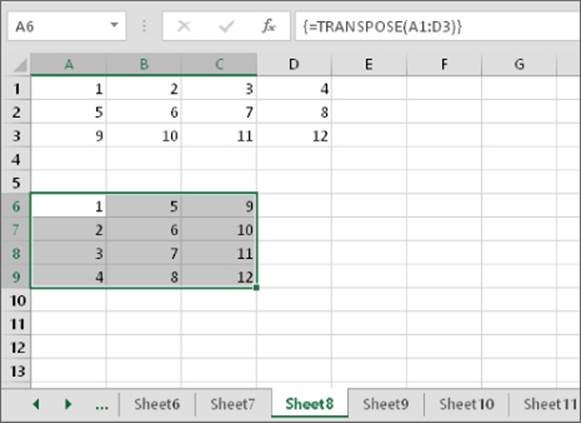
Figure 17.12 Using the TRANSPOSE function to transpose a rectangular array.
The formula in A6:C9 is
{=TRANSPOSE({1,2,3,4;5,6,7,8;9,10,11,12})}
You can, of course, use the TRANSPOSE function to transpose an array stored in a range. The following formula, for example, uses an array stored in A1:C4 (four rows, three columns). You can enter this array formula into a range that consists of three rows and four columns:
{=TRANSPOSE(A1:C4)}
Generating an array of consecutive integers
As you see in Chapter 18, generating an array of consecutive integers for use in a complex array formula is often useful. The ROW function, which returns a row number, is ideal for this. Consider the array formula shown here, entered into a vertical range of 12 cells:
{=ROW(1:12)}
This formula generates a 12-element array that contains integers from 1 to 12. To demonstrate, select a range that consists of 12 rows and one column and enter the array formula into the range. You'll find that the range is filled with 12 consecutive integers (as shown in Figure 17.13).
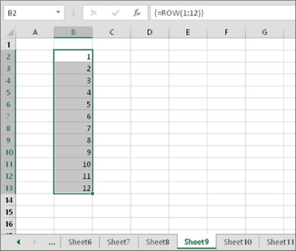
Figure 17.13 Using an array formula to generate consecutive integers.
If you want to generate an array of consecutive integers, a formula like the one shown previously is good — but not perfect. To see the problem, insert a new row above the range that contains the array formula. Excel adjusts the row references so that the array formula now reads
{=ROW(2:13)}
The formula that originally generated integers from 1 to 12 now generates integers from 2 to 13.
For a better solution, use this formula:
{=ROW(INDIRECT("1:12"))}
This formula uses the INDIRECT function, which takes a text string as its argument. Excel does not adjust the references contained in the argument for the INDIRECT function. Therefore, this array formula always returns integers from 1 to 12.
Chapter 18 contains several examples that use the technique for generating consecutive integers.
Worksheet Functions That Return an Array
Several of the Excel worksheet functions use arrays; you must enter into multiple cells a formula that uses one of these functions as an array formula. These functions are FORECAST, FREQUENCY, GROWTH, LINEST, LOGEST, MINVERSE, MMULT, and TREND. Consult the Excel Help system for more information.
Using Single-Cell Array Formulas
The examples in the preceding section all used a multicell array formula — a single array formula that's entered into a range of cells. The real power of using arrays becomes apparent when you use single-cell array formulas. This section contains examples of array formulas that occupy a single cell.
Counting characters in a range
Suppose that you have a range of cells that contains text entries (see Figure 17.14). If you need to get a count of the total number of characters in that range, the “traditional” method involves creating a formula like the one that follows and copying it down the column:
=LEN(A1)
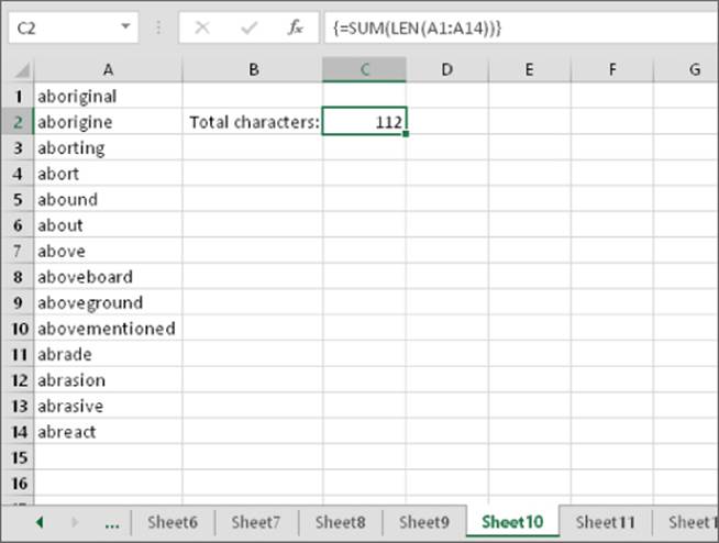
Figure 17.14 The goal is to count the number of characters in a range of text.
Then you use a SUM formula to calculate the sum of the values returned by these intermediate formulas.
The following array formula does the job without using any intermediate formulas:
{=SUM(LEN(A1:A14))}
The array formula uses the LEN function to create a new array (in memory) that consists of the number of characters in each cell of the range. In this case, the new array is
{10,9,8,5,6,5,5,10,11,14,6,8,8,7}
The array formula is then reduced to
=SUM({10,9,8,5,6,5,5,10,11,14,6,8,8,7})
The formula returns the sum of the array elements: 112.
Summing the three smallest values in a range
If you have values in a range named Data, you can determine the smallest value by using the SMALL function:
=SMALL(Data,1)
You can determine the second smallest and third smallest values by using these formulas:
=SMALL(Data,2)
=SMALL(Data,3)
To add the three smallest values, you can use a formula like this:
=SUM(SMALL(Data,1), SMALL(Data,2), SMALL(Data,3)
This formula works fine, but using an array formula is more efficient. The following array formula returns the sum of the three smallest values in a range named Data:
{=SUM(SMALL(Data,{1,2,3}))}
The formula uses an array constant as the second argument for the SMALL function. This generates a new array, which consists of the three smallest values in the range. This array is then passed to the SUM function, which returns the sum of the values in the new array.
Figure 17.15 shows an example in which the range A1:A10 is named Data. The SMALL function is evaluated three times, each time with a different second argument. The first time, the SMALL function has a second argument of 1, and it returns –5. The second time, the second argument for the SMALL function is 2, and it returns 0 (the second smallest value in the range). The third time, the SMALL function has a second argument of 3 and returns the third smallest value of 2.
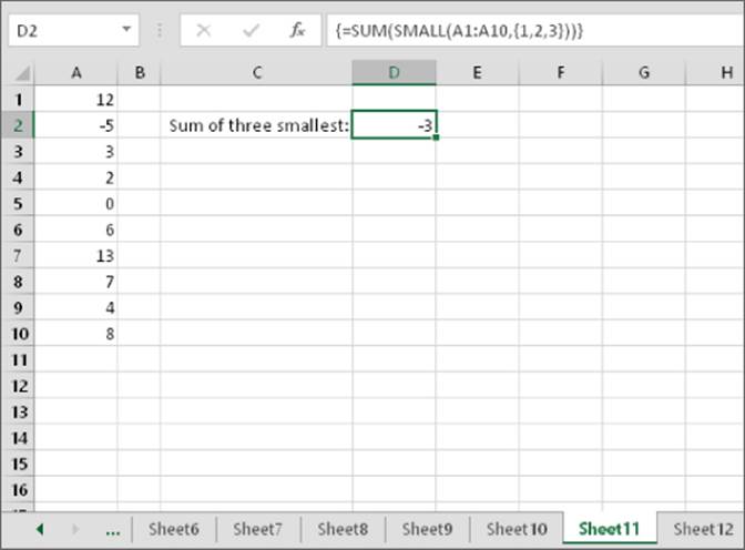
Figure 17.15 An array formula returns the sum of the three smallest values in A1:A10.
Therefore, the array that's passed to the SUM function is
{-5,0,2)
The formula returns the sum of the array (–3).
Counting text cells in a range
Suppose that you need to count the number of text cells in a range. The COUNTIF function seems like it might be useful for this task — but it's not. COUNTIF is useful only if you need to count values in a range that meet some criterion (for example, values greater than 12).
To count the number of text cells in a range, you need an array formula. The following array formula uses the IF function to examine each cell in a range. It then creates a new array (of the same size and dimensions as the original range) that consists of 1s and 0s, depending on whether the cell contains text. This new array is then passed to the SUM function, which returns the sum of the items in the array. The result is a count of the number of text cells in the range:
{=SUM(IF(ISTEXT(A1:D5),1,0))}
This general array formula type (that is, an IF function nested in a SUM function) is useful for counting. See Chapter 13, “Creating Formulas That Count and Sum,” for additional examples of IF and SUM functions.
Figure 17.16 shows an example of the preceding formula in cell C7. The array created by this formula is
{0,1,1,1;1,0,0,0;1,0,0,0;1,0,0,0;1,0,0,0}
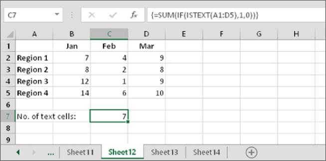
Figure 17.16 An array formula returns the number of text cells in the range.
Notice that this array contains four rows of three elements (the same dimensions as the range).
Here is a slightly more efficient variation on this formula:
{=SUM(ISTEXT(A1:D5)*1)}
This formula eliminates the need for the IF function and takes advantage of the fact that
TRUE * 1 = 1
and
FALSE * 1 = 0
Eliminating intermediate formulas
One key benefit of using an array formula is that you can often eliminate intermediate formulas in your worksheet, which makes your worksheet more compact and eliminates the need to display irrelevant calculations. Figure 17.17 shows a worksheet that contains pre-test and post-test scores for students. Column D contains formulas that calculate the changes between the pre-test and the post-test scores. Cell D17 contains a formula, shown here, that calculates the average of the values in column D:
=AVERAGE(D2:D15)
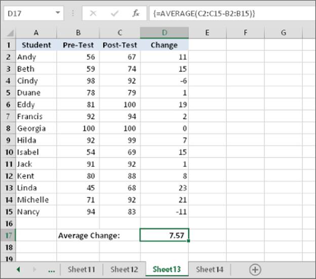
Figure 17.17 Without an array formula, calculating the average change requires intermediate formulas in column D.
With an array formula, you can eliminate column D. The following array formula calculates the average of the changes but does not require the formulas in column D:
{=AVERAGE(C2:C15-B2:B15)}
How does it work? The formula uses two arrays, the values of which are stored in two ranges (B2:B15 and C2:C15). The formula creates a new array that consists of the differences between each corresponding element in the other arrays. This new array is stored in Excel's memory, not in a range. The AVERAGE function then uses this new array as its argument and returns the result.
The new array, calculated from the two ranges, consists of the following elements:
{11,15,-6,1,19,2,0,7,15,1,8,23,21,-11}
The formula, therefore, is equivalent to this:
=AVERAGE({11,15,-6,1,19,2,0,7,15,1,8,23,21,-11})
Excel evaluates the function and displays the results, 7.57.
You can use additional array formulas to calculate other measures for the data in this example. For example, the following array formula returns the largest change (that is, the greatest improvement). This formula returns 23, which represents Linda's test scores.
{=MAX(C2:C15-B2:B15)}
The following array formula returns the smallest value in the Change column. This formula returns –11, which represents Nancy's test scores:
{=MIN(C2:C15-B2:B15)}
Using an array in lieu of a range reference
If your formula uses a function that requires a range reference, you may be able to replace that range reference with an array constant. This is useful in situations in which the values in the referenced range do not change.
Note
A notable exception to using an array constant in place of a range reference in a function is with the database functions that use a reference to a criteria range (for example, DSUM). Unfortunately, using an array constant instead of a reference to a criteria range does not work.
Figure 17.18 shows a worksheet that uses a lookup table to display a word that corresponds to an integer. For example, looking up a value of 9 returns Nine from the lookup table in D1:E10. The formula in cell C1 is
=VLOOKUP(B1,D1:E10,2,FALSE)
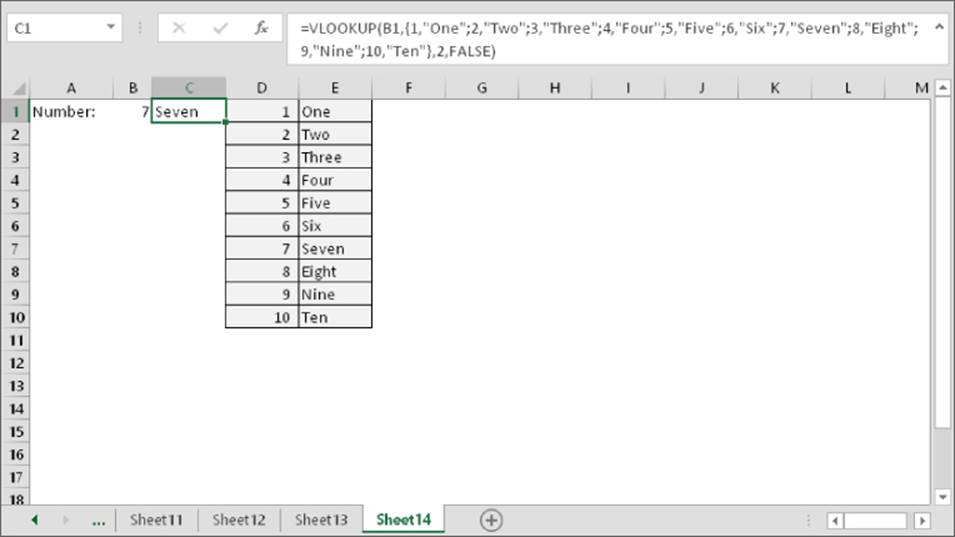
Figure 17.18 You can replace the lookup table in D1:E10 with an array constant.
For information about lookup formulas, see Chapter 14, “Creating Formulas That Look Up Values.”
You can use a two-dimensional array in place of the lookup range. The following formula returns the same result as the previous formula, but it does not require the lookup range in D1:E1:
=VLOOKUP(B1,{1,"One";2,"Two";3,"Three";4,"Four";5,"Five";6,"Six";7,"Seven";8,"Eight";9,"Nine";10,"Ten"},2,FALSE)
This chapter introduced arrays. Chapter 18 explores the topic further and provides some additional examples.
All materials on the site are licensed Creative Commons Attribution-Sharealike 3.0 Unported CC BY-SA 3.0 & GNU Free Documentation License (GFDL)
If you are the copyright holder of any material contained on our site and intend to remove it, please contact our site administrator for approval.
© 2016-2026 All site design rights belong to S.Y.A.