Microsoft Excel 2016 BIBLE (2016)

IN THIS CHAPTER

1. Introducing worksheet outlines

2. Creating an outline

3. Working with outlines

If you use a word processor, you may be familiar with the concept of an outline. Most word processors (including Microsoft Word) have an outline mode that lets you view only the headings and subheadings in your document. You can easily expand a heading to show the text below it. Using an outline makes visualizing the structure of your document easy.

Excel also is capable of using outlines. Understanding this feature can make working with certain types of worksheets much easier for you.

Introducing Worksheet Outlines

You'll find that some worksheets are more suitable for outlines than others. You can use outlines to create summary reports that don't show all the details. If your worksheet uses hierarchical data with subtotals, it's probably a good candidate for an outline.

The best way to understand how worksheet outlining works is to look at an example. Figure 27.1 shows a simple sales summary sheet without an outline. Formulas are used to calculate subtotals by region and by quarter.

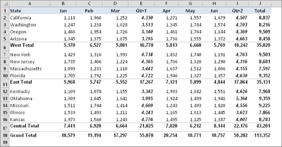
Figure 27.1 A simple sales summary with subtotals.

Figure 27.2 shows the same worksheet after I created the outline by selecting the rows and using Data Outline Group Auto Outline. Notice that Excel adds a new section to the left of the screen. This section contains outline controls that enable you to determine which level to view. This particular outline has three levels: States, Regions (each region consists of states grouped into categories such as West, East, and Central), and Grand Total (the sum of each region's subtotal).

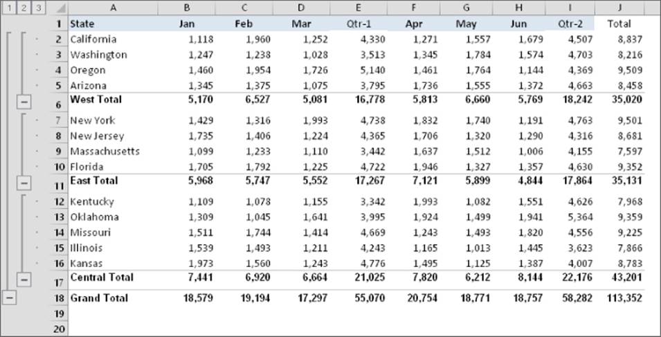
Figure 27.2 The worksheet after creating an outline.

Figure 27.3 depicts the outline after clicking the 2 button, which displays the second level of details. Now the outline shows only the totals for the regions. (The detail rows are hidden.) You can partially expand the outline to show the detail for a particular region by clicking one of the plus-sign buttons. Collapsing the outline to level 1 shows only the headers and the Grand Total row.

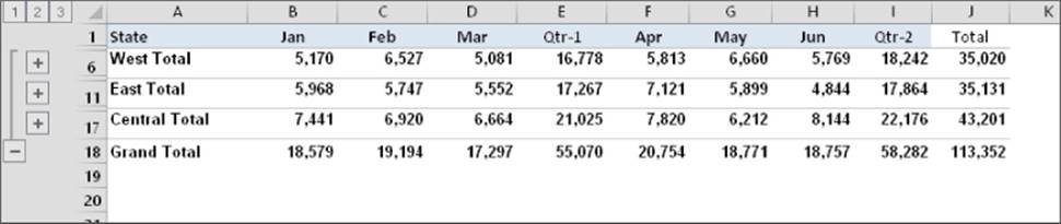
Figure 27.3 The worksheet after collapsing the outline to the second level.

Excel can create outlines in both directions. In the preceding examples, the outline is a row (vertical) outline. Figure 27.4 shows the same model after a column (horizontal) outline was added by selecting the columns and using Data Outline Group Auto Outline. When both outlines are in effect, Excel also displays outline controls at the top.

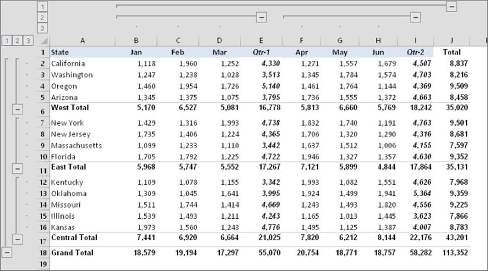
Figure 27.4 The worksheet after adding a column outline.

If you create both a row outline and a column outline in a worksheet, you can work with each outline independently of the other. For example, you can show the row outline at the second level and the column outline at the first level. Figure 27.5 shows the model with both outlines collapsed at the second level. The result is a high-level summary table that displays regional totals by quarter.

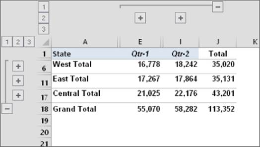
Figure 27.5 The worksheet with both outlines collapsed at the second level.

You can find the workbook used in the preceding examples on this book's website at www.wiley.com/go/excel2016bible. The file is named outline example.xlsx.

Keep in mind the following points about worksheet outlines:

· A worksheet can have only one outline. If you need to create more than one outline, use a different worksheet.

· You can either create an outline manually or have Excel do it for you automatically. If you choose the latter option, you may need to do some preparation to get the worksheet in the proper format. (The next section covers both methods.)

· You can create an outline either for all data on a worksheet or just for a selected data range.

· You can remove an outline with a single command: Data Outline Ungroup Clear Outline. See “Removing an outline,” later in this chapter.

· You can hide the outline symbols (to free screen space) but retain the outline. I show you how in the “Hiding the outline symbols” section, later in this chapter.

· An outline can have up to eight nested levels.

Worksheet outlines can be quite useful. If your main objective is to summarize a large amount of data, though, you may be better off using a pivot table. A pivot table is much more flexible and doesn't require that you create the subtotal formulas; it does the summarizing for you automatically. The ultimate solution depends on your data source. If you're entering data from scratch, the most flexible approach is to enter it in a normalized table format and create a pivot table.

I discuss pivot tables (and normalized data) in Chapter 33, “Introducing Pivot Tables,” and Chapter 34, “Analyzing Data with Pivot Tables.”

Creating an Outline

This section describes the two ways to create an outline: automatically and manually. Before you create an outline, you need to ensure that data is appropriate for an outline and that the formulas are set up properly.

Preparing the data

What type of data is appropriate for an outline? Generally, the data should be arranged in a hierarchy, such as a budget that consists of an arrangement similar to the following:

1. Company

1. Division

1. Department

1. Budget Category

1. Budget Item

In this case, each budget item (for example, airfare and hotel expenses) is part of a budget category (for example, travel expenses). Each department has its own budget, and the departments are rolled up into divisions. The divisions make up the company. This type of arrangement is well suited for a row outline.

The data arrangement suitable for an outline is essentially a summary table of your data. In some situations, your data will be “normalized” data — one data point per row. You can easily create a pivot table to summarize such data; a pivot table is much more flexible than an outline.

See Chapter 33 (“Introducing Pivot Tables”) and Chapter 34 (“Analyzing Data with Pivot Tables”) for more information about pivot tables.

After you create such an outline, you can view the information at any level of detail that you want by clicking the outline controls. When you need to create reports for different levels of management, consider using an outline. For example, upper management may want to see only the division totals, division managers may want to see totals by department, and each department manager needs to see the full details for his department.

Keep in mind that using an outline isn't a security feature. The data that's hidden when an outline is collapsed can easily be revealed when the outline is expanded.

You can include time-based information that is rolled up into larger units (such as months and quarters) in a column outline. Column outlines work just like row outlines, however, and the levels don't have to be time based.

Before you create an outline, you need to make sure that all the summary formulas are entered correctly and consistently. In this context, consistently means that the formulas are in the same relative location. Generally, formulas that compute summary formulas (such as subtotals) are entered below the data to which they refer. In some cases, however, the summary formulas are entered above the referenced cells. Excel can handle either method, but you must be consistent throughout the range that you outline. If the summary formulas aren't consistent, automatic outlining won't produce the results that you want.

Note

If your summary formulas aren't consistent (that is, some are above and some are below the data), you still can create an outline, but you must do it manually.

Creating an outline automatically

Excel can create an outline for you automatically in a few seconds, whereas it may take you ten minutes or more to do the same thing manually.

Note

If you've created a table for your data (by choosing Insert Tables Table), Excel can't create an outline automatically. You can create an outline from a table, but you must do so manually.

To have Excel create an outline, move the cell pointer anywhere within the range of data that you're outlining. Then, choose Data Outline Group Auto Outline. Excel analyzes the formulas in the range and creates the outline. Depending on the formulas that you have, Excel creates a row outline, a column outline, or both.

If the worksheet already has an outline, Excel asks whether you want to modify the existing outline. Click Yes to force Excel to remove the old outline and create a new one.

Note

Excel automatically creates an outline when you choose Data Outline Subtotal, which inserts subtotal formulas automatically.

Creating an outline manually

Usually, letting Excel create the outline is the best approach. It's much faster and less error prone. If the outline that Excel creates isn't what you have in mind, however, you can create one manually.

When Excel creates a row outline, the summary rows must all be below the data or all above the data; they can't be mixed. Similarly, for a column outline, the summary columns must all be to the right of the data or to the left of the data. If your worksheet doesn't meet these requirements, you have two choices:

· Rearrange the worksheet so that it does meet the requirements.

· Create the outline manually.

You also need to create an outline manually if the range doesn't contain formulas. You may have imported a file and want to use an outline to display it better. Because Excel uses the positioning of the formulas to determine how to create the outline, it can't make an outline without formulas.

Creating an outline manually consists of creating groups of rows (for row outlines) or groups of columns (for column outlines). To create a group of rows, follow these steps:

1. Select the rows that you want to include in the group. One way to do this is to click a row number and then drag to select other adjacent rows.

Caution

Don't select the row that has the summary formulas. You don't want these rows to be included in the group.

2. Choose Data Outline Group Group. Excel displays outline symbols for the group.

3. Repeat this process for each group that you want to create. When you collapse the outline, Excel hides rows in the group, but the summary row, which isn't in the group, remains in view.

Caution

If you select a range of cells (rather than entire rows or columns) before you create a group, Excel displays a dialog box asking what you want to group. It then groups entire rows or columns based on the range that you select.

You can also select groups of groups to create multilevel outlines. When you create multilevel outlines, always start with the innermost groupings and then work your way out. If you realize that you grouped the wrong rows, you can ungroup the group by selecting the rows and choosing Data Outline Ungroup Ungroup.

Here are keyboard shortcuts you can use that speed up grouping and ungrouping:

· Alt+Shift+right arrow: Groups selected rows or columns

· Alt+Shift+left arrow: Ungroups selected rows or columns

Creating outlines manually can be confusing at first, but if you stick with it, you'll become a pro in no time.

Figure 27.6 shows a worksheet with a three-level outline of this book. I had to create it manually because it has no formulas, just text.

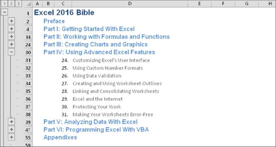
Figure 27.6 An outline of this book, created manually.

This workbook is available on this book's website at www.wiley.com/go/excel2016bible. The file is named book outline.xlsx.

Working with Outlines

This section discusses the basic operations that you can perform with a worksheet outline.

Displaying levels

To display various outline levels, click the appropriate outline symbol. These symbols consist of buttons with numbers on them (1, 2, and so on) or a plus sign (+) or minus sign (–). Refer to Figure 27.5, which shows these symbols for a row and column outline.

Clicking the 1 button collapses the outline so that it displays no detail (just the highest summary level of information), clicking the 2 button expands the outline to show one level, and so on. The number of numbered buttons depends on the number of outline levels. Choosing a level number displays the detail for that level, plus any levels with lower numbers. To display all levels (the most detail), click the highest-level number.

You can expand a particular section by clicking its plus-sign button, or you can collapse a particular section by clicking its minus-sign button. In short, you have complete control over the details that Excel exposes or hides in an outline.

If you prefer, you can use the Hide Detail and Show Detail commands on the Data Outline group to hide and show details, respectively.

Tip

If you constantly adjust the outline to show different reports, consider using the Custom Views feature to save a particular view and give it a name. Then you can quickly switch among the named views. Choose View Workbook Views Custom Views.

Adding data to an outline

You may need to add additional rows or columns to an outline. In some cases, you may be able to insert new rows or columns without disturbing the outline, and the new rows or columns become part of the outline. In other cases, you'll find that the new row or column is not part of the outline. If you create the outline automatically, choose Data Outline Group Auto Outline. Excel makes you verify that you want to modify the existing outline. If you create the outline manually, you need to make the adjustments manually as well.

Removing an outline

After you no longer need an outline, you can remove it by choosing Data Outline Ungroup Clear Outline. Excel fully expands the outline by displaying all hidden rows and columns, and the outline symbols disappear. Be careful before you remove an outline, however. You can't make it reappear by clicking the Undo button; you must re-create the outline from scratch.

Adjusting the outline symbols

When you create a manual outline, Excel puts the outline symbols below the summary rows. This can be unintuitive because you need to click the symbol in the row below the section that you want to expand.

If you prefer that the outline symbols appear in the same row as the summary row, click the dialog box launcher in the lower right of the Data Outline group. Excel displays the dialog box shown in Figure 27.7. Remove the check mark from the Summary Rows Below Detail option, and click OK. The outline will now display the outline symbols in a more logical position.

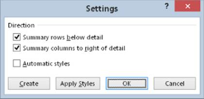
Figure 27.7 Use the Settings dialog box to adjust the position of the outline symbols.

Hiding the outline symbols

The outline symbols Excel displays when an outline is present take up quite a bit of space. (The exact amount depends on the number of levels.) If you want to see as much as possible onscreen, you can temporarily hide these symbols without removing the outline. Press Ctrl+8 to toggle the outline symbols on and off. When the outline symbols are hidden, you can't expand or collapse the outline.

Note

When you hide the outline symbols, the outline still is in effect, and the worksheet displays the data at the current outline level. (That is, some rows or columns may be hidden.)

The Custom Views feature, which saves named views of your outline, also saves the status of the outline symbols as part of the view, enabling you to name some views with the outline symbols and other views without them.