Microsoft Excel 2016 BIBLE (2016)

IN THIS CHAPTER

1. Using various methods to link workbooks

2. Consolidating multiple worksheets

In this chapter, I discuss two procedures that you might find helpful: linking and consolidating. Linking is the process of using references to cells in external workbooks to get data into your worksheet. Consolidating involves combining or summarizing information from two or more worksheets (which can be in multiple workbooks).

Linking Workbooks

As you may know, Excel allows you to create formulas that contain references to other workbook files. In such a case, the workbooks are linked in such a way that one depends on the other. The workbook that contains the external reference formulas is the dependentworkbook (because it contains formulas that depend on another workbook). The workbook that contains the information used in the external reference formula is the source workbook (because it's the source of the information).

When you consider linking workbooks, you may ask yourself the following question: if Workbook A needs to access data in another workbook (Workbook B), why not just enter the data into Workbook A in the first place? In some cases, you can. But the real value of linking becomes apparent when the source workbook is being continually updated by another person or group. Creating a link in Workbook A to Workbook B means that in Workbook A, you always have access to the most recent information in Workbook B because Workbook A is updated whenever Workbook B changes.

Linking workbooks also can be helpful if you need to consolidate different files. For example, each regional sales manager may store data in a separate workbook. You can create a summary workbook that first uses link formulas to retrieve specific data from each manager's workbook and then calculates totals across all regions.

Linking also is useful as a way to break up a large workbook into smaller files. You can create smaller workbooks that are linked with a few key external references.

Linking has its downside, however. External reference formulas are somewhat fragile, and accidentally severing the links that you create is relatively easy. You can prevent this mistake if you understand how linking works. Later in the chapter, I discuss some problems that may arise and how to avoid them. (See “Avoiding Potential Problems with External Reference Formulas.”)

The website for this book at www.wiley.com/go/excel2016bible contains two linked files that you can use to get a feel for the way linking works. The files are named source.xlsx and dependent.xlsx. As long as these files remain in the same folder, the links will be maintained.

Creating External Reference Formulas

You can create an external reference formula by using several different techniques:

· Type the cell references manually. These references may be lengthy because they include workbook and sheet names and possibly even drive and path information. These references can also point to workbooks stored on the Internet. The advantage of manually typing the cell references is that the source workbook doesn't have to be open. The disadvantage is that it's error prone. Mistyping a single character makes the formula return an error (or possibly return a wrong value from the workbook).

· Point to the cell references. If the source workbook is open, you can use the standard pointing techniques to create formulas that use external references.

· Paste the links. Copy your data to the Clipboard. Then, with the source workbook open, choose Home Clipboard Paste Paste Link (N). Excel pastes the copied data as external reference formulas.

· Choose Data Data Tools Consolidate. For more on this method, see the section “Consolidating worksheets by using the Consolidate dialog box,” later in this chapter.

Understanding link formula syntax

The general syntax for an external reference formula is as follows:

=[WorkbookName]SheetName!CellAddress

Precede the cell address with the workbook name (in brackets), followed by the worksheet name and an exclamation point. Here's an example of a formula that uses cell A1 in the Sheet1 worksheet of a workbook named Budget:

=[Budget.xlsx]Sheet1!A1

If the workbook name or the sheet name in the reference includes one or more spaces, you must enclose the text in single quotation marks. For example, here's a formula that refers to cell A1 on Sheet1 in a workbook named Annual Budget.xlsx:

='[Annual Budget.xlsx]Sheet1'!A1

When a formula links to a different workbook, you don't need to open the other workbook. However, if the workbook is closed and not in the current folder, you must add the complete path to the reference. For example:

='C:\Data\Excel\Budget\[Annual Budget.xlsx]Sheet1'!A1

If the workbook is stored on the Internet, the formula will also include the URL. For example:

='https://d.docs.live.net/86a6d7c1f41bd208/Documents/[Annual Budget.xlsx]Sheet1'!A1

Note

Single quotes are always required when the link includes a path or a URL, even if the path or URL includes no spaces.

Creating a link formula by pointing

Entering external reference formulas manually usually isn't the best approach because you can easily make an error. Instead, have Excel build the formula for you, as follows:

1. Open the source workbook.

2. Select the cell in the dependent workbook that will hold the formula.

3. Type an equal sign (=)

4. Activate the source workbook and select the cell or range and press Enter. The dependent workbook is reactivated.

When you point to the cell or range, Excel automatically takes care of the details and creates a syntactically correct external reference. When you're using this method, the cell reference is always an absolute reference (such as $A$1). If you plan to copy the formula to create additional link formulas, you need to change the absolute reference to a relative reference by removing the dollar signs for the cell address.

As long as the source workbook remains open, the external reference doesn't include the path (or URL) to the workbook. If you close the source workbook, however, the external reference formulas change to include the full path (or URL).

Pasting links

Pasting links provides another way to create external reference formulas. This method is applicable when you want to create formulas that simply reference other cells. Follow these steps:

1. Open the source workbook.

2. Select the cell or range that you want to link, and then copy it to the Clipboard. Ctrl+C is the quickest way.

3. Activate the dependent workbook and select the cell in which you want the link formula to appear. If you're pasting a copied range, just select the upper-left cell.

4. Choose Home Clipboard Paste Paste Link (N).

Working with External Reference Formulas

This section discusses some key points that you need to know about when working with links. Understanding these details can help prevent some common errors.

Creating links to unsaved workbooks

Excel enables you to create link formulas to unsaved workbooks (and even to nonexistent workbooks). Assume that you have two workbooks open (Book1 and Book2) and you haven't saved either of them. If you create a link formula to Book1 in Book2 and then save Book2, Excel displays a confirmation dialog box like the one shown in Figure 28.1.

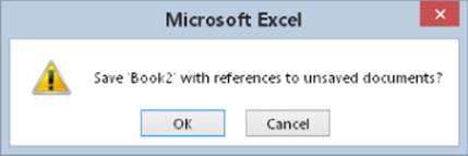
Figure 28.1 This confirmation message indicates that the workbook you're saving contains references to a workbook that you haven't yet saved.

Typically, you don't want to save a workbook that has links to an unsaved document. To avoid this prompt, save the source workbook first.

You can also create links to documents that don't exist. You may want to do so if you'll be using a source workbook from a colleague but the file hasn't yet arrived. When you enter an external reference formula that refers to a nonexistent workbook, Excel displays its Update Values dialog box, which resembles the Open dialog box. If you click Cancel, the formula retains the workbook name that you entered, but it returns a #REF! error.

When the source workbook becomes available, you can choose Data Connections Edit Links to update the link. (See “Updating links,” later in this chapter.) After doing so, the error goes away, and the formula displays its proper value.

Opening a workbook with external reference formulas

When you open a workbook that contains links, Excel displays a dialog box (shown in Figure 28.2) that asks you what to do. Your options are

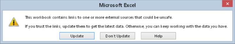
Figure 28.2 Excel displays this dialog box when you open a workbook that contains links to other files.

· Update: The links are updated with the current information in the source file(s).

· Don't Update: The links are not updated, and the workbook displays the previous values returned by the link formulas.

· Help: The Excel Help screen displays so you can read about links.

What if you choose to update the links but the source workbook is no longer available? If Excel can't locate a source workbook that's referred to in a link formula, it displays a dialog box with two choices:

· Continue: Open the workbook, but don't update the links.

· Edit Links: Display the Edit Links dialog box, shown in Figure 28.3. Click the Change Source button to specify a different workbook, or click the Break Link button to destroy the link and keep the current values.

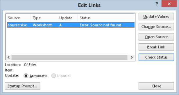
Figure 28.3 The Edit Links dialog box.

You can also access the Edit Links dialog box by choosing Data Connections Edit Links. The Edit Links dialog box lists all source workbooks, plus other types of links to other documents.

Tip

To prevent Excel from displaying the dialog box in Figure 28.2, open the Excel Options dialog box, select the Advanced tab, and remove the check mark from Ask to Update Automated Links. That disables the dialog box for all workbooks.

Changing the startup prompt

When you open a workbook that contains one or more external reference formulas, Excel, by default, displays the dialog box that asks how you want to handle the links (refer to Figure 28.2). You can eliminate this prompt by changing a setting in the Startup Prompt dialog box (see Figure 28.4).

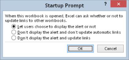
Figure 28.4 Use the Startup Prompt dialog box to specify how Excel handles links when the workbook is opened.

To display the Startup Prompt dialog box, choose Data Connections Edit Links. The Edit Links dialog box (refer to Figure 28.3) appears. In the Edit Links dialog box, click the Startup Prompt button and then select the option that describes how you want to handle the links.

Updating links

If you want to ensure that your link formulas have the latest values from their source workbooks, you can force an update. For example, say that you just discovered that someone made changes to the source workbook and saved the latest version to your network server. In such a case, you may want to update the links to display the current data.

To update linked formulas with their current value, open the Edit Links dialog box (Data Connections Edit Links), choose the appropriate source workbook in the list, and then click the Update Values button. Excel updates the link formulas with the latest version of the source workbook.

Note

Excel always sets worksheet links to the Automatic Update option in the Edit Links dialog box, and you can't change them to Manual, which means that Excel updates the links only when you open the workbook. Excel doesn't automatically update links when the source file changes (unless the source workbook is open).

Changing the link source

In some cases, you may need to change the source workbook for your external references. For example, say you have a worksheet that has links to a file named Preliminary Budget but you later receive a finalized version named Final Budget.

You can change the link source using the Edit Links dialog box (choose Data Connections Edit Links). Select the source workbook that you want to change, and click the Change Source button. Excel displays its Change Source dialog box, from which you can select a new source file. After you select the file, all external reference formulas that referred to the old file are updated.

Severing links

If you have external references in a workbook and then decide that you no longer need the links, you can convert the external reference formulas to values, thereby severing the links. To do so, access the Edit Links dialog box (choose Data Connections Edit Links), select the linked file in the list, and then click Break Link.

Caution

Excel prompts you to verify your intentions because you can't undo this operation.

Avoiding Potential Problems with External Reference Formulas

Using external reference formulas can be quite useful, but the links may be unintentionally severed. As long as the source file hasn't been deleted, you can almost always reestablish lost links. If you open the workbook and Excel can't locate the file, you see a dialog box that enables you to specify the workbook and re-create the links. You also can change the source file by clicking the Change Source button in the Edit Links dialog box (choose Data Connections Edit Links). The following sections discuss some pointers that you must remember when you use external reference formulas.

Renaming or moving a source workbook

If you or someone else renames the source document or moves it to a different folder, Excel won't be able to update the links. You need to use the Edit Links dialog box and specify the new source document. (See “Changing the link source,” earlier in this chapter.)

Note

If the source and dependent folder reside in the same folder, you can move both of the files to a different folder. In such a case, the links remain intact.

Using the Save As command

If both the source workbook and the dependent workbook are open, Excel doesn't display the full path to the source file in the external reference formulas. If you use the File Save As command to give the source workbook a new name, Excel modifies the external references to use the new workbook name. In some cases, this change may be what you want. But in other cases, it may not.

Here's an example of how using File Save As can cause a problem. You finished working on a source workbook and save the file. Then you decide to be safe and make a backup copy on a different drive, using File Save As. The formulas in the dependent workbook now refer to the backup copy, not the original source file. This is not what you want.

Bottom line? Be careful when you choose File Save As with a workbook that is the source of a link in another open workbook.

Modifying a source workbook

If you open a workbook that is a source workbook for another workbook, be extremely careful if the dependent workbook isn't open. For example, if you add a new row to the source workbook, all the cells move down one row. When you open the dependent workbook, it continues to use the old cell references, which is probably not what you want.

Note

It's easy to determine the source workbooks for a particular dependent workbook: just examine the files listed in the Edit Links dialog box (choose Data Connections Edit Links). However, it's not possible to determine whether a particular workbook is used as the source for another workbook.

You can avoid this problem by

· Always opening the dependent workbook(s) when you modify the source workbook: If you do so, Excel adjusts the external references in the dependent workbook when you make changes to the source workbook.

· Using names rather than cell references in your link formula: This approach is the safest.

The following link formula refers to cell C21 on Sheet1 in the budget.xlsx workbook:

=[budget.xlsx]Sheet1!$C$21

If cell C21 is named Total, you can write the formula using that name:

=budget.xlsx!Total

Using a name ensures that the link retrieves the correct value, even if you add or delete rows or columns from the source workbook.

By the way, notice that the filename isn't enclosed in brackets. That's because Total is assumed to be a workbook-level name and doesn't need to be qualified with a sheet name. If Total were a sheet-level name (defined on Sheet1), the formula would be this:

=[budget.xlsx]Sheet1!Total

See Chapter 4, “Working with Cells and Ranges,” for more information about creating names for cells and ranges.

Intermediary links

Excel doesn't place many limitations on the complexity of your network of external references. For example, Workbook A can contain external references that refer to Workbook B, which can contain an external reference that refers to Workbook C. In this case, a value in Workbook A can ultimately depend on a value in Workbook C. Workbook B is an intermediary link.

I don't recommend using intermediary links, but if you must use them, be aware that Excel doesn't update external reference formulas if the dependent workbook isn't open. In the preceding example, assume that Workbooks A and C are open. If you change a value in Workbook C, Workbook A won't reflect the change because you didn't open Workbook B (the intermediary link).

Consolidating Worksheets

The term consolidation, in the context of worksheets, refers to several operations that involve multiple worksheets or multiple workbook files. In some cases, consolidation involves creating link formulas. Here are two common examples of consolidation:

· The budget for each department in your company is stored in a single workbook, with a separate worksheet for each department. You need to consolidate the data and create a company-wide budget on a single sheet.

· Each department head submits a budget to you in a separate workbook file. Your job is to consolidate these files into a company-wide budget.

These types of tasks can be very difficult or quite easy. The task is easy if the information is laid out exactly the same in each worksheet. If the worksheets aren't laid out identically, they may be similar enough. In the second example, some budget files submitted to you may be missing categories that aren't used by a particular department. In this case, you can use a handy feature in Excel that matches data by using row and column titles. I discuss this feature in “Consolidating worksheets by using the Consolidate dialog box,” later in this chapter.

If the worksheets bear little or no resemblance to each other, your best option may be to edit the sheets so that they correspond to one another. Or return the files to the department heads and ask that they submit them using a standardized format. Better yet, redesign your workflow to use normalized tables that can be used as the source for pivot tables.

You can use any of the following techniques to consolidate information from multiple workbooks:

· Use external reference formulas.

· Copy the data, and choose Home Clipboard Paste Paste Link (N).

· Use the Consolidate dialog box, which you get to by choosing Data Data Tools Consolidate.

Time to Rethink Your Consolidation Strategy?

If you're reading this chapter, there's a good chance you're looking for a way to combine data from multiple sources. The consolidation methods I describe can work, but they may not be the most efficient way to approach the problem.

A typical budget is actually a summary. It's usually much easier to work with “normalized” data, which consists of one row per data item. Then you can use Excel's most sophisticated tool (a pivot table) to consolidate and summarize the information.

For example, a budget for Region 1 might show a value for training expenses for the IT department for January. Instead of just entering this number into a grid, you gain a lot of flexibility by putting it into a table with multiple columns that describe the number. For example, this single item can be represented as a row in a normalized table with these six headings: Region, Department, Expense Description, Month, Year, and Budget Amount.

If each regional manager submitted his budget information in this format, it would be a simple matter to combine the data in a single worksheet and then create a pivot table that displays a summary in just about any layout you want.

Consolidating worksheets by using formulas

Consolidating with formulas simply involves creating formulas that use references to other worksheets or other workbooks. Here are the primary advantages to using this method of consolidation:

· If the values in the source worksheets change, the formulas are updated automatically.

· The source workbooks don't need to be open when you create the consolidation formulas.

If you're consolidating the worksheets in the same workbook and all the worksheets are laid out identically, the consolidation task is simple. You can just use standard formulas to create the consolidations. For example, to compute the total for cell A1 in worksheets named Sheet2 through Sheet10, enter the following formula:

=SUM(Sheet2:Sheet10!A1)

You can enter this formula manually or use the multisheet selection technique. You can then copy this formula to create summary formulas for other cells.

See Chapter 4, for more on multisheet selection.

If the consolidation involves other workbooks, you can use external reference formulas to perform your consolidation. For example, if you want to add the values in cell A1 from Sheet1 in two workbooks (named Region1 and Region2), you can use the following formula:

=[Region1.xlsx]Sheet1!B2+[Region2.xlsx]Sheet1!B2

You can include any number of external references in this formula, up to the 8,000-character limit for a formula. However, if you use many external references, such a formula can be quite lengthy and confusing if you need to edit it.

If the worksheets that you're consolidating aren't laid out the same, you can still use formulas, but you need to ensure that each formula refers to the correct cell — a task that is both tedious and error prone.

Consolidating worksheets by using Paste Special

Another method of consolidating information is to use the Paste Special dialog box. This technique takes advantage of the fact that the Paste Special dialog box can perform a mathematical operation when it pastes data from the Clipboard. For example, you can use the Add option to add the copied data to the selected range. Figure 28.5 shows the Paste Special dialog box.

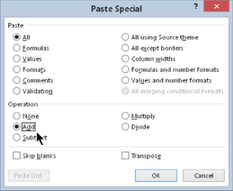
Figure 28.5 Choosing the Add operation in the Paste Special dialog box.

This method is applicable only when all the worksheets that you're consolidating are open. The disadvantage is that the consolidation isn't dynamic. In other words, it doesn't generate formulas that refer to the original source data. So, if any data that was consolidated changes, the consolidation is no longer accurate.

Here's how to use this method:

1. Copy the data from the first source range.

2. Activate the dependent workbook and select a location for the consolidated data. A single cell is sufficient.

3. Choose Home Clipboard Paste Paste Special. The Paste Special dialog box appears.

4. Choose the Values option and the Add operation, and then click OK.

Repeat these steps for each source range that you want to consolidate. Make sure that the consolidation location in Step 2 is the same for each paste operation.

Caution

This method is probably the worst way of consolidating data. It can be rather error prone, and the lack of formulas means that there is no “trail.” If an error is discovered, it may be difficult or impossible to determine the source of the error.

Consolidating worksheets by using the Consolidate dialog box

For the ultimate in data consolidation, use the Consolidate dialog box. This method is flexible, and in some cases, it even works if the source worksheets aren't laid out identically. This technique can create consolidations that are static (no link formulas) or dynamic(with link formulas). The Data Consolidate feature supports the following methods of consolidation:

· By position: This method is accurate only if the worksheets are laid out identically.

· By category: Excel uses row and column labels to match data in the source worksheets. Use this option if the data is laid out differently in the source worksheets or if some source worksheets are missing rows or columns.

Figure 28.6 shows the Consolidate dialog box, which appears when you choose Data Data Tools Consolidate.

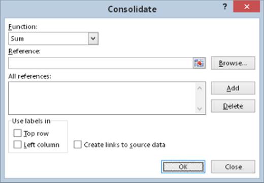
Figure 28.6 The Consolidate dialog box enables you to specify ranges to consolidate.

Following is a description of the controls in this dialog box:

· Function drop-down list: Specify the type of consolidation. Sum is the most commonly used consolidation function, but you can also select from ten other options.

· Reference box: Specify a range from a source file that you want to consolidate. You can enter the range reference manually or use any standard pointing technique (if the workbook is open). Named ranges are also acceptable. After you enter the range in this box, click Add to add it to the All References list. If you consolidate by position, don't include labels in the range; if you consolidate by category, do include labels in the range.

· All References list box: This contains the list of references that you've added with the Add button.

· Use Labels In check boxes: Use this to instruct Excel to perform the consolidation by examining the labels in the top row, the left column, or both positions. Use these options when you consolidate by category.

· Create Links to Source Data check box: When you select this option, Excel adds summary formulas for each label and creates an outline. If you don't select this option, the consolidation doesn't use formulas, and an outline isn't created.

· Browse button: Click to display a dialog box that enables you to select a workbook to open. It inserts the filename in the Reference box, but you have to supply the range reference. You'll find that your job is much easier if all the workbooks to be consolidated are open.

· Add button: Click to add the reference in the Reference box to the All References list. Make sure that you click this button after you specify each range.

· Delete button: Click to delete the selected reference from the All References list.

A workbook consolidation example

The simple example in this section demonstrates the power of the Data Consolidate feature. Figure 28.7 shows three single-sheet workbooks that will be consolidated. These worksheets report three months of product sales. Notice, however, that all don't report on the same products. In addition, the products aren't listed in the same order. In other words, these worksheets aren't laid out identically. Creating consolidation formulas manually would be a tedious task.

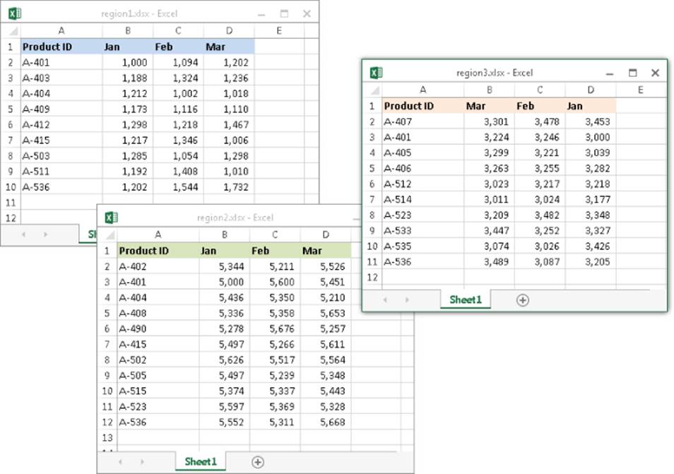
Figure 28.7 Three worksheets to be consolidated.

These workbooks are available on this book's website at www.wiley.com/go/excel2016bible. The files are named region1.xlsx, region2.xlsx, and region3.xlsx.

To consolidate this information, start with a new workbook. You don't need to open the source workbooks, but consolidation is easier if they're open. Follow these steps to consolidate the workbooks:

1. Choose Data Data Tools Consolidate. The Consolidate dialog box appears.

2. Select the type of consolidation summary that you want to use from the Function drop-down list. Use Sum for this example.

3. Enter the reference for the first worksheet to consolidate. If the workbook is open, you can point to the reference; if it isn't open, click the Browse button to locate the file on disk. The reference must include a range. You can use a range that includes complete columns, such as A:K. This range is larger than the actual range to consolidate, but using this range ensures that the consolidation will still work if new rows and columns are added to the source file. When the reference in the Reference box is correct, click Add to add it to the All References list.

4. Enter the reference for the second worksheet. You can point to the range in the Region2 workbook, or you can simply edit the existing reference by changing Region1 to Region2 and then clicking Add. This reference is added to the All References list.

5. Enter the reference for the third worksheet. Again, you can edit the existing reference by changing Region2 to Region3 and then clicking Add. This final reference is added to the All References list.

6. Because the worksheets aren't laid out the same, select the Left Column and the Top Row check boxes to force Excel to match the data by using the labels.

7. Select the Create Links to Source Data check box to make Excel create an outline with external references.

8. Click OK to begin the consolidation.

Excel creates the consolidation, beginning at the active cell. Notice that Excel created an outline, which is collapsed to show only the subtotals for each product. If you expand the outline (by clicking the number 2 or the plus-sign symbols in the outline), you can see the details. Examine it further, and you discover that each detail cell is an external reference formula that uses the appropriate cell in the source file. Therefore, the consolidated results are updated automatically when values are changed in any of the source workbooks.

Figure 28.8 shows the result of the consolidation, and Figure 28.9 shows the summary information (with the outline collapsed to hide the details).

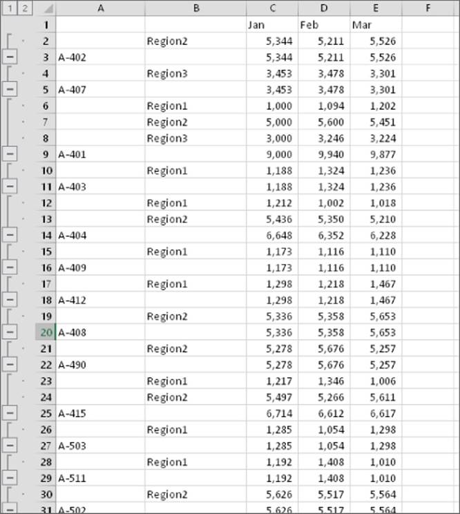
Figure 28.8 The result of consolidating the information in three workbooks.

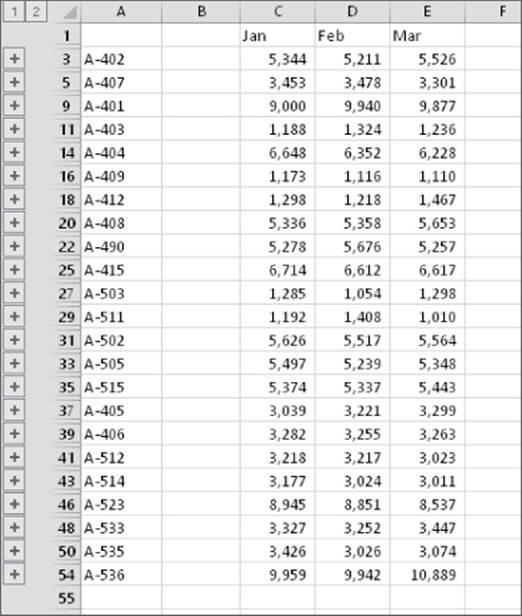
Figure 28.9 Collapsing the outline to show only the totals.

For more information on Excel outlines, see Chapter 27, “Creating and Using Worksheet Outlines.”

Refreshing a consolidation

When you choose the option to create formulas, the external references in the consolidation workbook are created only for data that exists at the time of the consolidation. Therefore, if new rows are added to any of the original workbooks, the consolidation must be redone. Fortunately, the consolidation parameters are stored with the workbook, so it's a simple matter to rerun the consolidation if necessary. That's why specifying complete columns and including extra columns (in Step 3 in the preceding section) is a good idea.

Excel remembers the references that you entered in the Consolidate dialog box and saves them with the workbook. That way, if you want to refresh a consolidation, you won't have to reenter the references. Just display the Consolidate dialog box, verify that the ranges are correct, and then click OK.

More about consolidation

Excel is flexible regarding the sources that you can consolidate. You can consolidate data from the following:

· Open workbooks.

· Closed workbooks. You need to enter the reference manually, but you can use the Browse button to get the filename part of the reference.

· The same workbook in which you're creating the consolidation.

And, of course, you can mix and match any of the preceding choices in a single consolidation.

If you perform the consolidation by matching labels, be aware that the matches must be exact. For example, Jan doesn't match January. The matching is not case sensitive, however, so April does match APRIL. In addition, the labels can be in any order, and they don't need to be in the same order in all the source ranges.

If you don't select the Create Links to Source Data check box, Excel generates a static consolidation. (It doesn't create formulas.) Therefore, if the data on any of the source worksheets changes, the consolidation won't update automatically. To update the summary information, you need to choose Data Data Tools Consolidate again.

If you do select the Create Links to Source Data check box, Excel creates a standard worksheet outline that you can manipulate by using the techniques described in Chapter 27.