Microsoft Excel 2016 BIBLE (2016)

IN THIS CHAPTER

1. Considering a what-if example

2. Identifying types of what-if analyses

3. Looking at manual what-if analyses

4. Creating one-input and two-input data tables

5. Using Scenario Manager

One of the most appealing aspects of Excel is its ability to create dynamic models. A dynamic model uses formulas that instantly recalculate when you change values in cells that are used by the formulas. When you change values in cells in a systematic manner and observe the effects on specific formula cells, you're performing a type of what-if analysis.

What-if analysis is the process of asking such questions as “What if the interest rate on the loan changes to 7.5% rather than 7.0%?” and “What if we raise our product prices by 5%?”

If you set up your worksheet properly, answering such questions is simply a matter of plugging in new values and observing the results of the recalculation. Excel provides useful tools to assist you in your what-if endeavors.

A What-If Example

Figure 35.1 shows a simple worksheet model that calculates information pertaining to a mortgage loan. The worksheet is divided into two sections: the input cells and the result cells (which contain formulas).

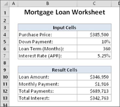
Figure 35.1 This simple worksheet model uses four input cells to produce the results.

This workbook is available on this book's website at www.wiley.com/go/excel2016bible. The filename is mortgage loan.xlsx.

With this worksheet, you can easily answer the following what-if questions:

· What if I can negotiate a lower purchase price on the property?

· What if the lender requires a 20% down payment?

· What if I can get a 40-year mortgage?

· What if the interest rate increases to 5.50%?

You can answer these questions by simply changing the values in the cells in range C4:C7 and observing the effects in the dependent cells (C10:C13). You can, of course, vary any number of input cells simultaneously.

Avoid Hard-Coding Values in a Formula

The mortgage calculation example, simple as it is, demonstrates an important point about spreadsheet design: you should always set up your worksheet so that you have maximum flexibility to make changes. Perhaps the most fundamental rule of spreadsheet design is the following:

· Do not hard-code values in a formula. Instead, store the values in separate cells and use cell references in the formula.

The term hard-code refers to the use of actual values, or constants, in a formula. In the mortgage loan example, all the formulas use references to cells, not actual values.

You could use the value 360, for example, for the loan term argument of the pmt function in cell C11 of Figure 35.1. Using a cell reference has two advantages. First, you have no doubt about the values that the formula uses. (They aren't buried in the formula.) Second, you can easily change the value — which is easier than editing the formula.

Using values in formulas may not seem like much of an issue when only one formula is involved, but just imagine what would happen if this value were hard-coded into several hundred formulas that were scattered throughout a worksheet.

Types of What-If Analyses

Not surprisingly, Excel can handle much more sophisticated models than the preceding example. To perform a what-if analysis using Excel, you have three basic options:

· Manual what-if analysis: Plug in new values and observe the effects on formula cells.

· Data tables: Create a special type of table that displays the results of selected formula cells as you systematically change one or two input cells.

· Scenario Manager: Create named scenarios and generate reports that use outlines or pivot tables.

I discuss each of these types of what-if analysis in the rest of this chapter.

Performing manual what-if analysis

A manual what-if analysis doesn't require too much explanation. In fact, the example that opens this chapter demonstrates how it's done. Manual what-if analysis is based on the idea that you have one or more input cells that affect one or more key formula cells. You change the value in the input cells and observe the formula calculations. You may want to print the results or save each scenario to a new workbook. The term scenario refers to a specific set of values in one or more input cells.

Manual what-if analysis is common. People often use this technique without even realizing that they're doing a type of what-if analysis. This method of performing what-if analysis certainly has nothing wrong with it, but you should be aware of some other techniques.

If your input cells are not located near the formula cells, consider using a Watch Window to monitor the formula results in a movable window. I discuss this feature in Chapter 3, “Essential Worksheet Operations.”

Creating data tables

This section describes one of Excel's most underutilized features: data tables. A data table is a dynamic range that summarizes formula cells for varying input cells. You can create a data table fairly easily, but data tables have some limitations. In particular, a data table can deal with only one or two input cells at a time. This limitation becomes clear as you view the examples.

Note

Scenario Manager, discussed later in this chapter (see “Using Scenario Manager”), can produce a report that summarizes any number of input cells and result cells.

Don't confuse a data table with a standard table (created by choosing Insert Tables Table). These two features are completely independent.

Creating a one-input data table

A one-input data table displays the results of one or more formulas for various values of a single input cell. Figure 35.2 shows the general layout for a one-input data table. You need to set up the table yourself, manually. This is not something that Excel will do for you.

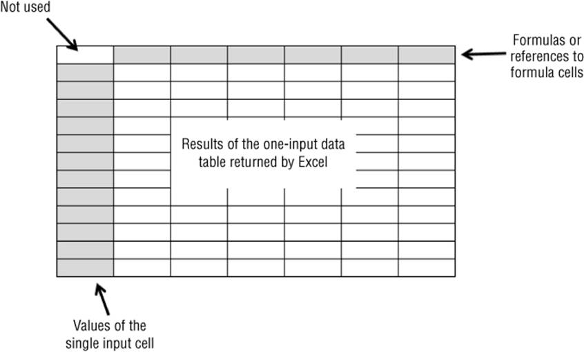
Figure 35.2 How a one-input data table is set up.

You can place the data table anywhere in a worksheet. The left column contains various values for the single input cell. The top row contains references to formulas located elsewhere in the worksheet. You can use a single formula reference or any number of formula references. The upper-left cell of the table remains empty. Excel calculates the values that result from each value of the input cell and places them under each formula reference.

This example uses the mortgage loan worksheet from earlier in the chapter (see “A What-If Example”). The goal of this exercise is to create a data table that shows the values of the four formula cells (loan amount, monthly payment, total payments, and total interest) for various interest rates ranging from 4.5% to 6.5%, in 0.25% increments.

This workbook is available on this book's website at www.wiley.com/go/excel2016bible. The file is named mortgage loan data table.xlsx.

Figure 35.3 shows the setup for the data table area. Row 3 consists of references to the formulas in the worksheet. For example, cell F3 contains the formula =C10, and cell G3 contains the formula =C11. Row 2 contains optional descriptive labels, and these are not actually part of the data table. Column E contains the values of the single input cell (interest rate) that Excel will use in the table.

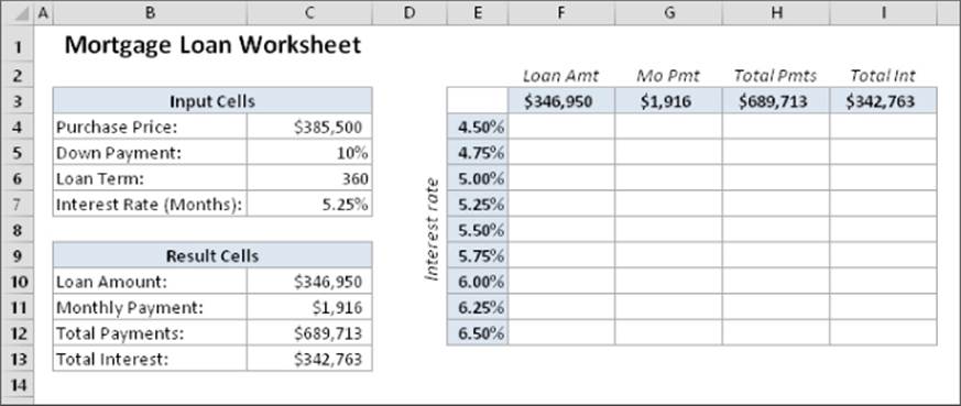
Figure 35.3 Preparing to create a one-input data table.

To create the table, select the entire data table range (in this case, E3:I12) and then choose Data Forecast What-If Analysis Data Table. The Data Table dialog box, shown in Figure 35.4, appears.

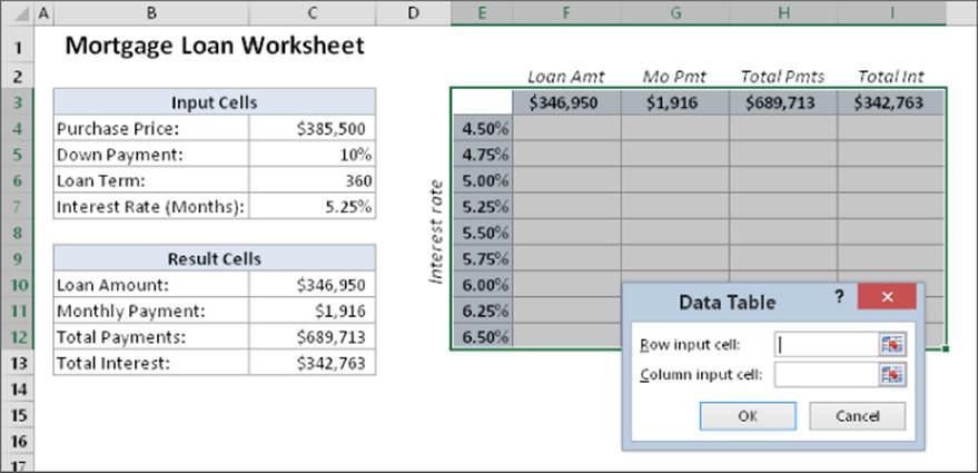
Figure 35.4 The Data Table dialog box.

You must specify the worksheet cell that contains the input value. Because variables for the input cell appear in the left column in the data table, you place this cell reference in the Column Input Cell field. Enter C7 or point to the cell in the worksheet. Leave the Row Input Cell field blank. Click OK, and Excel fills in the table with the calculated results (see Figure 35.5).

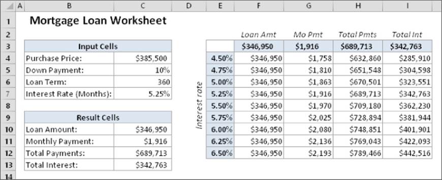
Figure 35.5 The result of the one-input data table.

Caution

For some reason, using the Data Table command wipes out Excel's undo stack. So operations that you perform prior to using this command cannot be undone.

Using this table, you can now see the calculated loan values for varying interest rates. Notice that the Loan Amt column (column F) doesn't vary. That's because the formula in cell C10 doesn't depend on the interest rate.

If you examine the contents of the cells that Excel entered as a result of this command, you'll see that the data is generated with a multicell array formula:

{=TABLE(,C7)}

As I discuss in Chapter 17, “Introducing Array Formulas,” a multicell array formula is a single formula that can produce results in multiple cells. Because the table uses formulas, Excel updates the table that you produce if you change the cell references in the first row or plug in different interest rates in the first column.

Note

You can arrange a one-input table vertically (as in this example) or horizontally. If you place the values of the input cell in a row, you enter the input cell reference in the Row Input Cell field of the Data Table dialog box.

Creating a two-input data table

As the name implies, a two-input data table lets you vary two input cells. You can see the setup for this type of table in Figure 35.6. Although it looks similar to a one-input table, the two-input table has one critical difference: it can show the results of only one formula at a time. With a one-input table, you can place any number of formulas, or references to formulas, across the top row of the table. In a two-input table, this top row holds the values for the second input cell. The upper-left cell of the table contains a reference to the single result formula.

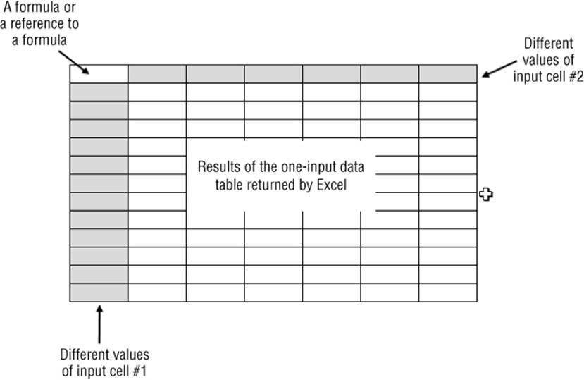
Figure 35.6 The setup for a two-input data table.

Using the mortgage loan worksheet, you could create a two-input data table that shows the results of a formula (say, monthly payment) for various combinations of two input cells (such as interest rate and down-payment percent). To see the effects on other formulas, you simply create multiple data tables — one for each formula cell that you want to summarize.

The example in this section uses the worksheet shown in Figure 35.7 to demonstrate a two-input data table. In this example, a company wants to conduct a direct-mail promotion to sell its product. The worksheet calculates the net profit from the promotion.

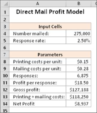
Figure 35.7 This worksheet calculates the net profit from a direct-mail promotion.

This workbook, named direct mail data table.xlsx, is on this book's website at www.wiley.com/go/excel2016bible.

This model uses two input cells: the number of promotional pieces mailed and the anticipated response rate. The following items appear in the Parameters area:

· Printing costs per unit: The cost to print a single mailer. The unit cost varies with the quantity: $0.20 each for quantities less than 200,000; $0.15 each for quantities of 200,001 through 300,000; and $0.10 each for quantities of more than 300,000. The following formula is used:

=IF(B4<200000,0.2,IF(B4<300000,0.15,0.1))

· Mailing costs per unit: A fixed cost, $0.28 per unit mailed.

· Responses: The number of responses, calculated from the response rate and the number mailed. The formula in this cell is the following:

=B4*B5

· Profit per response: A fixed value. The company knows that it will realize an average profit of $18.50 per order.

· Gross profit: This is a simple formula that multiplies the profit-per-response by the number of responses:

=B10*B11

· Print + mailing costs: This formula calculates the total cost of the promotion:

=B4*(B8+B9)

· Net Profit: This formula calculates the bottom line — the gross profit minus the printing and mailing costs.

If you enter values for the two input cells, you see that the net profit varies quite a bit, often going negative to produce a net loss.

Figure 35.8 shows the setup of a two-input data table that summarizes the net profit at various combinations of quantity and response rate; the table appears in the range E4:M14. Cell E4 contains a formula that references the Net Profit cell:

=B14

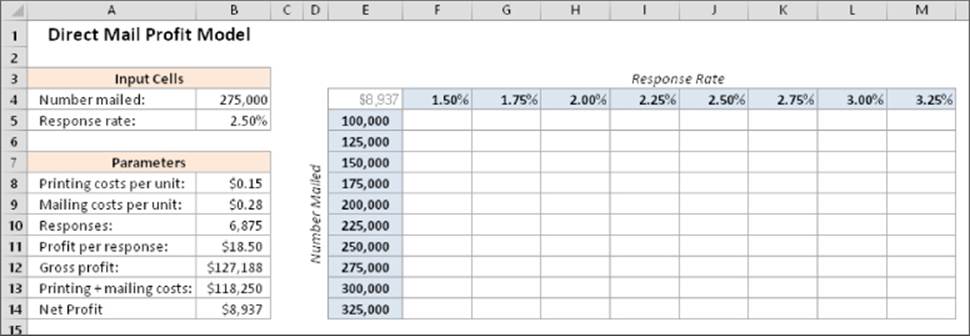
Figure 35.8 Preparing to create a two-input data table.

To create the data table, follow these steps:

1. Enter the response rate values in F4:M4.

2. Enter the number mailed values in E5:E14.

3. Select the range E4:M14 and choose Data Forecast What-If Analysis Data Table. The Data Table dialog box appears.

4. Specify B5 as the Row input cell (the response rate) and B4 as the Column input (the number mailed).

5. Click OK. Excel fills in the data table.

Figure 35.9 shows the result. As you can see, quite a few of the combinations of response rate and quantity mailed result in a loss rather than a profit.

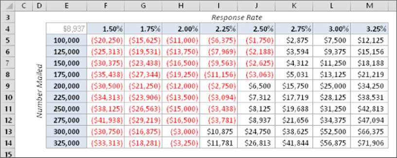
Figure 35.9 The result of the two-input data table.

As with the one-input data table, this data table is dynamic. You can change the formula in cell E4 to refer to another cell (such as gross profit). Or you can enter some different values for Response Rate and Number Mailed.

Using Scenario Manager

Data tables are useful, but they have a few limitations:

· You can vary only one or two input cells at a time.

· Setting up a data table is not intuitive.

· A two-input table shows the results of only one formula cell (although you can create additional tables for more formulas).

· In many situations, you're interested in a few select combinations, not an entire table that shows all possible combinations of two input cells.

The Scenario Manager is a fairly easy way to automate some aspects of your what-if models. You can store different sets of input values (called changing cells in the terminology of Scenario Manager) for any number of variables and give a name to each set. You can then select a set of values by name, and Excel displays the worksheet by using those values. You can also generate a summary report that shows the effect of various combinations of values on any number of result cells. These summary reports can be an outline or a pivot table.

For example, your annual sales forecast may depend on several factors. Consequently, you can define three scenarios: best case, worst case, and most likely case. You then can switch to any of these scenarios by selecting the named scenario from a list. Excel substitutes the appropriate input values in your worksheet and recalculates the formulas.

Defining scenarios

To introduce you to Scenario Manager, this section starts with an example that uses a simplified production model, as shown in Figure 35.10.

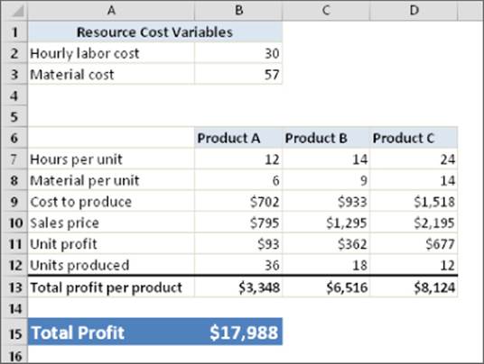
Figure 35.10 A simple production model to demonstrate Scenario Manager.

This workbook, named production model scenarios.xlsx, is available on this book's website at www.wiley.com/go/excel2016bible.

This worksheet contains two input cells: the hourly labor cost (cell B2) and the unit cost for materials (cell B3). The company produces three products, and each product requires a different number of hours and a different amount of materials to produce.

Formulas calculate the total profit per product (row 13) and the total combined profit (cell B15). Management — trying to predict the total profit, but uncertain what the hourly labor cost and material costs will be — has identified three scenarios, listed in Table 35.1.

Table 35.1 Three Scenarios for the Production Model

The Best Case scenario has the lowest hourly cost and the lowest materials cost. The Worst Case scenario has high values for both the hourly cost and the materials cost. The third scenario, Most Likely Case, has intermediate values for both of these input cells. The managers need to be prepared for the worst case, however, and they're interested in what would happen under the Best Case scenario.

Choose Data Forecast What-If Analysis Scenario Manager to display the Scenario Manager dialog box. When you first open this dialog box, it tells you that no scenarios are defined — which is not too surprising because you're just starting. As you add named scenarios, they appear in the Scenarios list in this dialog box.

Tip

It's a good idea to create names for the changing cells and all the result cells that you want to examine. Excel uses these names in the dialog boxes and in the reports that it generates. If you use names, keeping track of what's going on is much easier; names also make your reports more readable.

To add a scenario, click the Add button in the Scenario Manager dialog box. Excel displays its Add Scenario dialog box, shown in Figure 35.11.

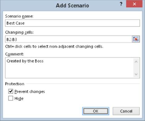
Figure 35.11 Use the Add Scenario dialog box to create a named scenario.

This dialog box consists of four parts:

· Scenario Name: You can give the scenario any name that you like.

· Changing Cells: These are the input cells for the scenario. You can enter the cell addresses directly or point to them. If you've created a name for the cells, type the name. Nonadjacent cells are allowed; if pointing to multiple cells, press Ctrl while you click the cells. Each named scenario can use the same set of changing cells or different changing cells. The number of changing cells for a scenario is limited to 32.

· Comment: By default, Excel displays the name of the person who created the scenario and the date when it was created. You can change this text, add new text to it, or delete it.

· Protection: The two Protection options (preventing changes and hiding a scenario) are in effect only when you protect the worksheet and choose the Scenario option in the Protect Sheet dialog box. Protecting a scenario prevents anyone from modifying it; a hidden scenario doesn't appear in the Scenario Manager dialog box.

In this example, define the three scenarios that are listed in Table 36.1. The changing cells are Hourly cost (B2) and Materials cost (B3).

After you enter the information in the Add Scenario dialog box, click OK. Excel then displays the Scenario Values dialog box, shown in Figure 35.12. This dialog box displays one field for each changing cell that you specified in the previous dialog box. Enter the values for each cell in the scenario. If you click OK, you return to the Scenario Manager dialog box, which then displays your named scenario in its list. If you have more scenarios to create, click the Add button to return to the Add Scenario dialog box.

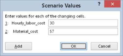
Figure 35.12 You enter the values for the scenario in the Scenario Values dialog box.

Displaying scenarios

After you define all the scenarios and return to the Scenario Manager dialog box, the dialog box displays the names of your defined scenarios. Select one of the scenarios and then click the Show button (or double-click the Scenario name). Excel inserts the corresponding values into the changing cells and calculates the worksheet to show the results for that scenario. Figure 35.13 shows an example of selecting a scenario.

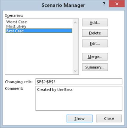
Figure 35.13 Selecting a scenario to display.

Using the Scenarios Drop-Down List

The Scenarios drop-down list shows all the defined scenarios and enables you to quickly display a scenario. Oddly, this useful tool doesn't appear on the Ribbon. But if you use Scenario Manager, you can add the Scenarios control to your Quick Access toolbar. Here's how:

1. Right-click the Quick Access toolbar and choose Customize Quick Access Toolbar from the shortcut menu. The Excel Options dialog box appears, with the Quick Access Toolbar tab selected.

2. From the Choose Commands From drop-down list, select Commands Not in the Ribbon.

3. Scroll down the list and select Scenario.

4. Click the Add button.

5. Click OK to close the Excel Options dialog box.

Alternatively, you can add the Scenarios control to the Ribbon. See Chapter 24, “Customizing the Excel User Interface,” for additional details on customizing the Quick Access toolbar and the Ribbon.

Moodifying scenarios

After you've created scenarios, you may need to change them. To do so, follow these steps:

1. Click the Edit button in the Scenario Manager dialog box to change one or more of the values for the changing cells of a scenario.

2. From the Scenarios list, select the scenario that you want to change and then click the Edit button. The Edit Scenario dialog box appears.

3. Click OK. The Scenario Values dialog box appears.

4. Make your changes and then click OK to return to the Scenario Manager dialog box. Notice that Excel automatically updates the Comments box with new text that indicates when the scenario was modified.

Merging scenarios

In workgroup situations, you may have several people working on a spreadsheet model, and several people may have defined various scenarios. The marketing department, for example, may have its opinion of what the input cells should be, the finance department may have another opinion, and your CEO may have yet another opinion.

Excel makes it easy to merge these various scenarios into a single workbook. Before you merge scenarios, make sure that the workbook from which you're merging is open:

1. Click the Merge button in the Scenario Manager dialog box.

2. From the Merge Scenarios dialog box that appears, choose the workbook that contains the scenarios you're merging in the Book drop-down list.

3. Choose the sheet that contains the scenarios you want to merge from the Sheet list box, and click Add. Notice that the dialog box displays the number of scenarios in each sheet as you scroll through the Sheet list box.

4. Click OK. You return to the previous dialog box, which now displays the scenario names that you merged from the other workbook.

Generating a scenario report

If you've created multiple scenarios, you may want to document your work by creating a scenario summary report. When you click the Summary button in the Scenario Manager dialog box, Excel displays the Scenario Summary dialog box.

You have a choice of report types:

· Scenario Summary: The summary report appears in the form of a worksheet outline.

· Scenario PivotTable: The summary report appears in the form of a pivot table.

See Chapter 27, “Creating and Using Worksheet Outlines,” for more information about outlines and Chapter 33, “Introducing Pivot Tables,” for an introduction to pivot tables.

For simple cases of scenario management, a standard Scenario Summary report is usually sufficient. If you have many scenarios defined with multiple result cells, however, you may find that a Scenario PivotTable provides more flexibility.

The Scenario Summary dialog box also asks you to specify the result cells (the cells that contain the formulas in which you're interested). For this example, select B13:D13 and B15 (a multiple selection) to make the report show the profit for each product, plus the total profit.

Note

As you work with Scenario Manager, you may discover its main limitation: namely, that a scenario can use no more than 32 changing cells. If you attempt to use more cells, you get an error message.

Excel creates a new worksheet to store the summary table. Figure 35.14 shows the Scenario Summary form of the report. If you gave names to the changing cells and result cells, the table uses these names; otherwise, it lists the cell references.

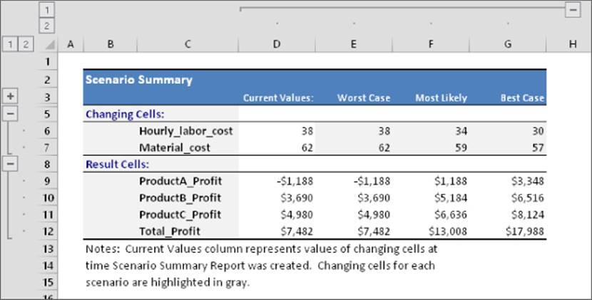
Figure 35.14 A Scenario Summary report produced by Scenario Manager.