Microsoft Excel 2016 BIBLE (2016)

IN THIS CHAPTER

1. Understanding how formatting can improve your worksheets

2. Getting to know the formatting tools

3. Using formatting in your worksheets

4. Using named styles for easier formatting

5. Understanding document themes

Formatting your worksheet is like the icing on a cake — it may not be absolutely necessary, but it can make the end product a lot more attractive. In an Excel worksheet, formatting can also make it easier for others to understand the worksheet's purpose.

Stylistic formatting isn't essential for every workbook that you develop — especially if it's for your own use only. On the other hand, it takes only a few moments to apply some simple formatting, and, after you apply it, the formatting will remain in place without further effort on your part.

In Chapter 5, “Introducing Tables,” I showed how easy it is to apply formatting to a table. The information in this chapter applies to normal ranges. I show you how to work with the Excel formatting tools: fonts, colors, and styles such as bold and italic. I also cover custom styles that you can create to make formatting large amounts of material in a similar way easier.

Getting to Know the Formatting Tools

Figure 6.1 shows how even simple formatting can significantly improve a worksheet's readability. The unformatted worksheet (on the left) is perfectly functional but not very readable compared to the formatted worksheet (on the right).

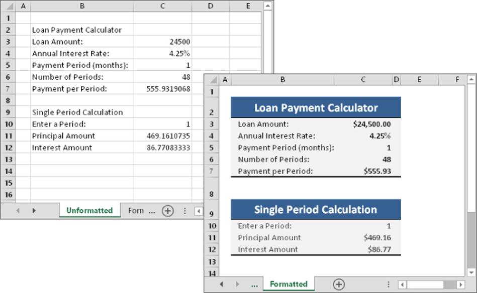
Figure 6.1 In just a few minutes, some simple formatting can greatly improve the appearance of your worksheet.

This workbook is available on this book's website at www.wiley.com/go/excel2016bible. The file is named loan payments.xlsx.

The Excel cell formatting tools are available in three locations:

· On the Home tab of the Ribbon

· On the Mini toolbar that appears when you right-click a selected range or a cell

· From the Format Cells dialog box

In addition, many common formatting commands have keyboard shortcuts.

Excel also enables you to format cells based on the cell's contents. Chapter 21, “Visualizing Data Using Conditional Formatting,” discusses conditional formatting.

Using the formatting tools on the Home tab

The Home tab of the Ribbon provides quick access to the most commonly used formatting options. Start by selecting the cell or range. Then, use the appropriate tool in the Font, Alignment, or Number groups.

Using these tools is intuitive, and the best way to familiarize yourself with them is to experiment. Enter some data, select some cells, and then click the controls to change the appearance. Note that some of these controls are actually drop-down lists. Click the small arrow on the button, and the button expands to display your choices.

Using the Mini toolbar

When you right-click a cell or a range selection, you get a shortcut menu. In addition, the Mini toolbar appears above or below the shortcut menu. Figure 6.2 shows how this toolbar looks. The Mini toolbar for cell formatting contains the most commonly used controls from the Home tab of the Ribbon.

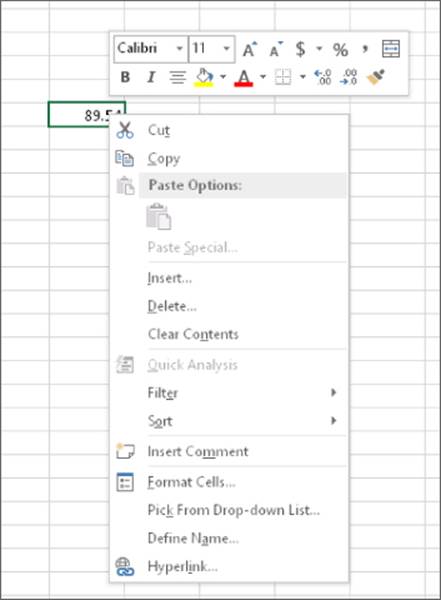
Figure 6.2 The Mini toolbar appears above or below the right-click shortcut menu.

If you use a tool on the Mini toolbar, the shortcut menu disappears, but the toolbar remains visible so you can apply other formatting to the selected cells. To hide the Mini toolbar, just click in any cell or press Escape.

Some people find the Mini toolbar distracting. Unfortunately, Excel doesn't provide a direct way to turn it off. If you really want to get rid of the Mini Toolbar, see the following sidebar, “Mini Toolbar Be Gone.”

Mini Toolbar Be Gone

If you find the Mini toolbar annoying, you can search all day and not find an option to turn it off. The General tab of the Excel Options dialog box has an option labeled Show Mini Toolbar on Selection, but this option applies to selecting characters while editing a cell. The only way to turn off the Mini toolbar when you right-click is to execute a VBA macro:

Sub ZapMiniToolbar()

Application.ShowMenuFloaties = True

End Sub

If you execute this VBA macro, the result is persistent. In other words, the Mini toolbar will not appear, even if you close and restart Excel. The only way to get the Mini toolbar back is to execute another VBA statement that sets the ShowMenuFloatiesproperty to False.

By the way, the statement might seem wrong, but it works. Contrary to what you would think, setting that property to True turns off the Mini toolbar. It's a bug that appeared in Excel 2007 and was not fixed in subsequent versions because correcting it would cause many macros to fail. (See Part VI, “Programming Excel with VBA,” for more information about VBA macros.)

Using the Format Cells dialog box

The formatting controls available on the Home tab of the Ribbon are sufficient most of the time, but some types of formatting require that you use the Format Cells dialog box. This tabbed dialog box lets you apply nearly any type of stylistic formatting and number formatting. The formats that you choose in the Format Cells dialog box apply to the cells that you have selected at the time. Later sections in this chapter cover the tabs of the Format Cells dialog box.

Note

When you use the Format Cells dialog box, you don't see the effects of your formatting choices until you click OK. With every new release of Excel, I expect to see the Format Cells dialog box implemented as a more convenient task pane. But I'm always disappointed. Maybe next time.

After selecting the cell or range to format, you can display the Format Cells dialog box by using any of the following methods:

· Press Ctrl+1.

· Click the dialog box launcher in Home Font, Home Alignment, or Home Number. (The dialog box launcher is the small downward-pointing arrow icon displayed to the right of the group name in the Ribbon.) When you display the Format Cells dialog box using a dialog box launcher, the dialog box is displayed with the appropriate tab visible.

· Right-click the selected cell or range and choose Format Cells from the shortcut menu.

· Click the More command in some of the drop-down controls in the Ribbon. For example, the Home Font Border More Borders drop-down includes an item named More Borders.

The Format Cells dialog box contains six tabs: Number, Alignment, Font, Border, Fill, and Protection. The following sections contain more information about the formatting options available in this dialog box.

Using Different Fonts to Format Your Worksheet

You can use different fonts, sizes, or text attributes in your worksheets to make various parts — such as the headers for a table — stand out. You also can adjust the font size. For example, using a smaller font allows for more information on a single screen or printed page.

By default, Excel uses 11-point (pt) Calibri font. A font is described by its typeface (Calibri, Cambria, Arial, Times New Roman, Courier New, and so on) as well as by its size, measured in points. (Seventy-two points equal one inch.) Excel's row height, by default, is 15 pt. Therefore, 11-pt type entered into 15-pt rows leaves a small amount of blank space between the characters in vertically adjacent rows.

Tip

If you haven't manually changed a row's height, Excel automatically adjusts the row height based on the tallest text that you enter into the row.

Updating Old Fonts

Office 2007 introduced several new fonts, and the default font has been changed for all the Office applications in subsequent releases. In versions prior to Excel 2007, the default font was 10 pt Arial. In Excel 2007 and later, the default font for the Office theme is 11 pt Calibri. Most people will agree that Calibri is much easier to read, and it gives the worksheet a more modern appearance.

If you open a workbook created in a pre-2007 version of Excel, the default font will not be changed, even if you apply a document style (by choosing Page Layout Themes Themes). But here's an easy way to update the fonts in a workbook that was created using an older version of Excel:

1. Press Ctrl+N to open a new, empty workbook. The new workbook will use the default document theme.

2. Open your old workbook file.

3. Choose Home Styles Cell Styles Merge Styles. Excel displays its Merge Styles dialog box.

4. In the Merge Styles dialog box, select the new workbook that you created in step 1.

5. Click OK.

6. Click Yes in response to Excel's question regarding merging styles that have the same name.

This technique changes the font and size for all unformatted cells. If you've applied font formatting to some cells (for example, made them bold), the font for those cells will not be changed (but you can change the font manually for those cells). If you don't like the new look of your workbook, just close the workbook without saving the changes.

Tip

If you plan to distribute a workbook to other users, remember that Excel does not embed fonts. Therefore, you should stick with the standard fonts that are included with Windows or Microsoft Office. If you open a workbook and your system doesn't have the font used in the workbook, Windows attempts to use a similar font. Sometimes this attempt works okay, and sometimes it doesn't.

Use the Font and Font Size tools on the Home tab of the Ribbon (or on the Mini toolbar) to change the font or size for selected cells.

You also can use the Font tab in the Format Cells dialog box to choose fonts, as shown in Figure 6.3. This tab enables you to control several other font attributes that aren't available elsewhere. Besides choosing the font, you can change the font style (bold, italic), underlining, color, and effects (strikethrough, superscript, or subscript). If you select the Normal Font check box, Excel displays the selections for the font defined for the Normal style. I discuss styles later in this chapter (see “Using Named Styles for Easier Formatting”).

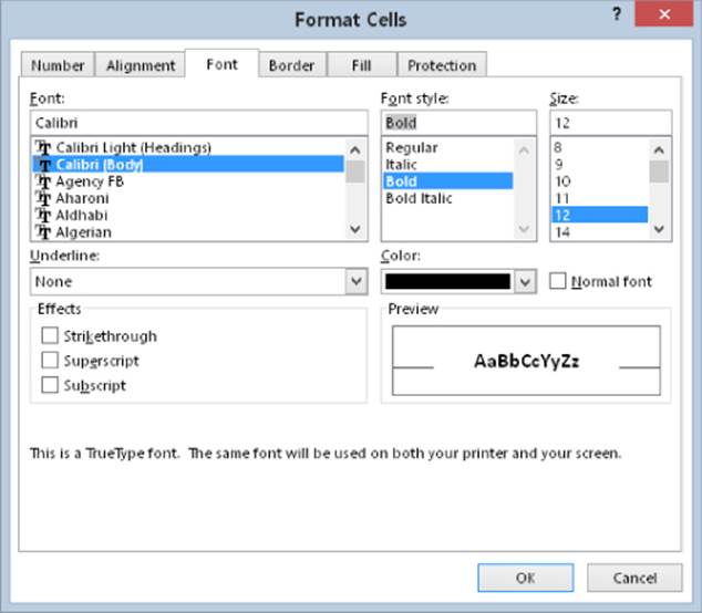
Figure 6.3 The Font tab of the Format Cells dialog box gives you many additional font attribute options.

Figure 6.4 shows several examples of font formatting. In this figure, gridlines were turned off to make the underlining more visible. Notice, in the figure, that Excel provides four different underlining styles. In the two nonaccounting underline styles, only the cell contents are underlined. In the two accounting underline styles, the entire width of the cells is always underlined.

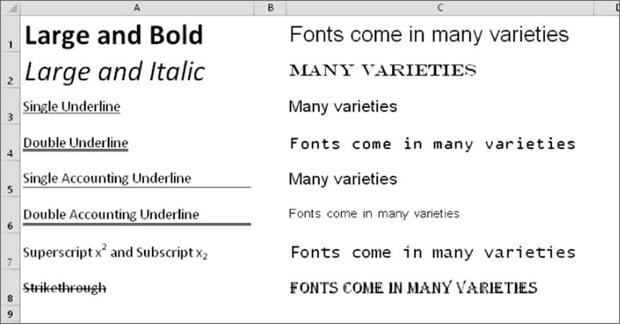
Figure 6.4 You can choose many different font formatting options for your worksheets.

If you prefer to keep both hands on the keyboard, you can use the following shortcut keys to format a selected range quickly:

· Ctrl+B: Bold

· Ctrl+I: Italic

· Ctrl+U: Underline

· Ctrl+5: Strikethrough

These shortcut keys act as a toggle. For example, you can turn bold on and off by repeatedly pressing Ctrl+B.

Using Multiple Formatting Styles in a Single Cell

If a cell contains text (as opposed to a value or a formula), you can apply formatting to individual characters in the cell. To do so, switch to Edit mode (press F2, or double-click the cell) and then select the characters that you want to format. You can select characters either by dragging the mouse over them or by pressing the Shift key as you press the left or right arrow key.

This technique is useful if you need to apply superscript or subscript formatting to a few characters in the cell (refer to Figure 6.4 for examples).

After you select the characters to format, use any of the standard formatting techniques, including options in the Format Cells dialog box. To display the Format Cells dialog box when editing a cell, press Ctrl+1. The changes apply only to the selected characters in the cell. This technique doesn't work with cells that contain values or formulas.

Changing Text Alignment

The contents of a cell can be aligned horizontally and vertically. By default, Excel aligns numbers to the right and text to the left. All cells use bottom alignment by default.

Overriding these defaults is a simple matter. The most commonly used alignment commands are in the Alignment group on the Home tab of the Ribbon. Use the Alignment tab of the Format Cells dialog box for even more options (see Figure 6.5).

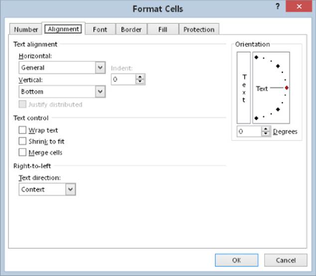
Figure 6.5 The full range of alignment options is available on the Alignment tab of the Format Cells dialog box.

Choosing horizontal alignment options

Horizontal alignment options, which control how cell contents are distributed across the width of the cell (or cells), are available from the Format Cells dialog box:

· General: Aligns numbers to the right, aligns text to the left, and centers logical and error values. This option is the default alignment.

· Left: Aligns the cell contents to the left side of the cell. If the text is wider than the cell, the text spills over to the cell on the right. If the cell on the right isn't empty, the text is truncated and not completely visible. Also available on the Ribbon.

· Center: Centers the cell contents in the cell. If the text is wider than the cell, the text spills over to cells on either side if they're empty. If the adjacent cells aren't empty, the text is truncated and not completely visible. Also available on the Ribbon.

· Right: Aligns the cell contents to the right side of the cell. If the text is wider than the cell, the text spills over to the cell on the left. If the cell on the left isn't empty, the text is truncated and not completely visible. Also available on the Ribbon.

· Fill: Repeats the contents of the cell until the cell's width is filled. If cells to the right also are formatted with Fill alignment, they also are filled.

· Justify: Justifies the text to the left and right of the cell. This option is applicable only if the cell is formatted as wrapped text and uses more than one line.

· Center across Selection: Centers the text over the selected columns. This option is useful for centering a heading over a number of columns.

· Distributed: Distributes the text evenly across the selected column.

Note

If you choose Left, Right, or Distributed, you can also adjust the Indent setting, which adds horizontal space between the cell border and the text.

Figure 6.6 shows examples of text that uses three types of horizontal alignment: Left, Justify, and Distributed (with an indent).

Figure 6.6 The same text, displayed with three types of horizontal alignment.

If you want to experiment with text alignment settings, this workbook is available at this book's website at www.wiley.com/go/excel2016bible. The file is named text alignment.xlsx.

Choosing vertical alignment options

Vertical alignment options typically aren't used as often as horizontal alignment options. In fact, these settings are useful only if you've adjusted row heights so that they're considerably taller than normal.

Here are the vertical alignment options available in the Format Cells dialog box:

· Top: Aligns the cell contents to the top of the cell. Also available on the Ribbon.

· Center: Centers the cell contents vertically in the cell. Also available on the Ribbon.

· Bottom: Aligns the cell contents to the bottom of the cell. Also available on the Ribbon.

· Justify: Justifies the text vertically in the cell; this option is applicable only if the cell is formatted as wrapped text and uses more than one line. This setting can be used to increase the line spacing.

· Distributed: Distributes the text evenly vertically in the cell.

Wrapping or shrinking text to fit the cell

If you have text too wide to fit the column width but you don't want that text to spill over into adjacent cells, you can use either the Wrap Text option or the Shrink to Fit option to accommodate that text. The Wrap Text option is also available on the Ribbon.

The Wrap Text option displays the text on multiple lines in the cell, if necessary. Use this option to display lengthy headings without having to make the columns too wide and without reducing the size of the text.

The Shrink to Fit option reduces the size of the text so that it fits into the cell without spilling over to the next cell. I've never had much luck with this command. Unless the text is just slightly too long, the result is almost always illegible.

Note

If you apply Wrap Text formatting to a cell, you can't use the Shrink to Fit formatting.

Merging worksheet cells to create additional text space

A handy formatting option is the ability to merge two or more cells. When you merge cells, you don't combine the contents of cells. Rather, you combine a group of cells into a single cell that occupies the same space. The worksheet shown in Figure 6.7 contains four sets of merged cells. Range C2:I2 has been merged into a single cell, and so have ranges J2:P2, B4:B8, and B9:B13. In the latter two cases, the text direction has also been changed (see “Displaying text at an angle,” later in this chapter).

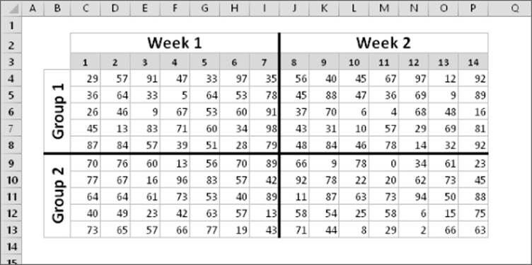
Figure 6.7 Merge worksheet cells to make them act as if they were a single cell.

You can merge any number of cells occupying any number of rows and columns. In fact, you can merge all 17,179,869,184 cells in a worksheet into a single cell — although I can't think of any good reason to do so, except maybe to play a trick on a coworker.

The range that you intend to merge should be empty, except for the upper-left cell. If any of the other cells that you intend to merge are not empty, Excel displays a warning. If you continue, all the data (except in the upper-left cell) will be deleted.

You can use the Alignment tab of the Format Cells dialog box to merge cells, but using the Merge & Center control on the Ribbon (or on the Mini toolbar) is simpler. To merge cells, select the cells that you want to merge and then click the Merge & Center button. The cells will be merged, and the content in the upper-left cells will be centered horizontally. The Merge & Center button acts as a toggle. To unmerge cells, select the merged cells and click the Merge & Center button again.

After you merge cells, you can change the alignment to something other than Center by using the controls in the Home Alignment group.

The Home Alignment Merge & Center control contains a drop-down list with these additional options:

· Merge Across: When a multirow range is selected, this command creates multiple merged cells — one for each row.

· Merge Cells: Merges the selected cells without applying the Center attribute.

· Unmerge Cells: Unmerges the selected cells.

Displaying text at an angle

In some cases, you may want to create more visual impact by displaying text at an angle within a cell. You can display text horizontally, vertically, or at any angle between 90 degrees up and 90 degrees down.

From the Home Alignment Orientation drop-down list, you can apply the most common text angles. For more control, use the Alignment tab of the Format Cells dialog box. In the Format Cells dialog box (refer to Figure 6.5), use the Degrees spinner control — or just drag the pointer in the gauge. You can specify a text angle between –90 and +90 degrees.

Figure 6.8 shows an example of text displayed at a 45-degree angle.

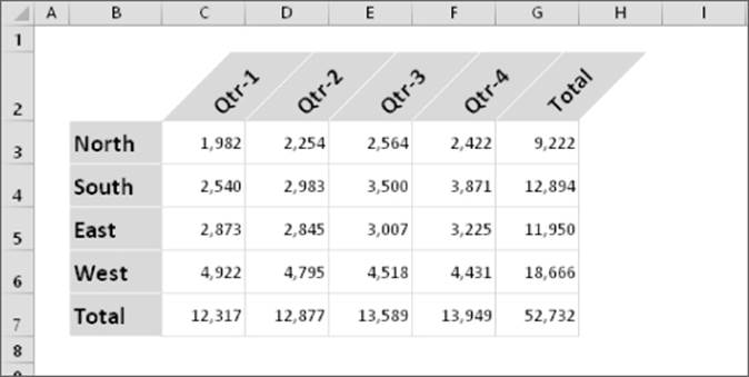
Figure 6.8 Rotate text for additional visual impact.

Note

Rotated text may look a bit distorted onscreen, but the printed output is usually of much better quality.

Controlling the text direction

Not all languages use the same character direction. Although most Western languages are read left to right, other languages are read right to left. You can use the Text Direction option to select the appropriate setting for the language you use. This command is available only in the Alignment tab of the Format Cells dialog box.

Don't confuse the Text Direction setting with the Orientation setting (discussed in the previous section). Changing the text orientation is common. Changing the text direction is used only in specific situations.

Note

Changing the Text Direction setting won't have any effect unless you have the proper language drivers installed on your system. For example, you must install Japanese language support to use right-to-left text direction Japanese characters. Use the Language tab of the Excel Options dialog box to determine which languages are installed.

Using Colors and Shading

Excel provides the tools to create some colorful worksheets. You can change the color of the text or add colors to the backgrounds of the worksheet cells. Prior to Excel 2007, workbooks were limited to a palette of 56 colors. Subsequent versions allow a virtually unlimited number of colors.

You control the color of the cell's text by choosing Home Font Font Color. Control the cell's background color by choosing Home Font Fill Color. Both of these color controls are also available on the Mini toolbar, which appears when you right-click a cell or range.

Tip

To hide the contents of a cell, make the background color the same as the font text color. The cell contents are still visible in the Formula bar when you select the cell. Keep in mind, however, that some printers may override this setting, and the text may be visible when printed.

Even though you have access to an unlimited number of colors, you might want to stick with the ten theme colors (and their light/dark variations) displayed in the various color selection controls. In other words, avoid using the More Color option, which lets you select a color. Why? First of all, those ten colors were chosen because they “go together.” (Well, at least somebody thought they did.) Another reason involves document themes. If you switch to a different document theme for your workbook, nontheme colors aren't changed. In some cases, the result may be less than pleasing, aesthetically. (See “Understanding Document Themes,” later in this chapter, for more information about themes.)

Using Colors with Table Styles

In Chapter 5, I discuss the handy Table feature. One advantage to using tables is that it's easy to apply table styles. You can change the look of your table with a single mouse click.

It's important to understand how table styles work with existing formatting. A simple rule is that applying a style to a table doesn't override existing formatting. For example, assume that you have a range of data that uses yellow as the background color for the cells. When you convert that range to a table (by choosing Insert Tables Table), the default table style (alternating row colors) isn't visible. Instead, the table will display the previously applied yellow background.

To make table styles visible with this table, you need to remove the manually applied background cell colors. Select the entire table and then choose Home Font Fill Color No Fill.

You can apply any type of formatting to a table, and that formatting will override the table style formatting. For example, you may want to make a particular cell stand out by using a different fill color.

Adding Borders and Lines

Borders (and lines within the borders) are another visual enhancement that you can add around groups of cells. Borders are often used to group a range of similar cells or to delineate rows or columns. Excel offers 13 preset styles of borders, as you can see in the Home Font Borders drop-down list shown in Figure 6.9. This control works with the selected cell or range and enables you to specify which, if any, border style to use for each border of the selection.

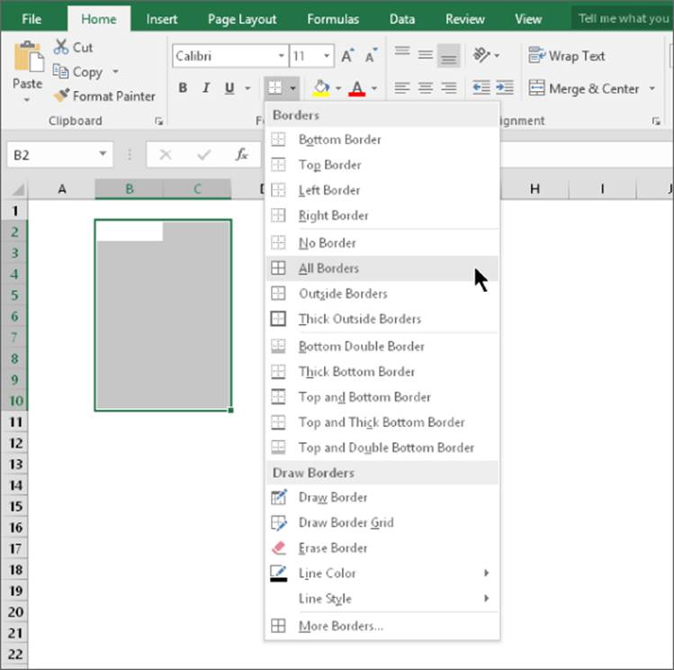
Figure 6.9 Use the Borders drop-down list to add lines around worksheet cells.

You may prefer to draw borders rather than select a preset border style. To do so, use the Draw Border or Draw Border Grid command from the Home Font Borders drop-down list. Selecting either command lets you create borders by dragging your mouse. Use the Line Color or Line Style command to change the color or style. When you're finished drawing borders, press Esc to cancel the border-drawing mode.

Another way to apply borders is to use the Border tab of the Format Cells dialog box, which is shown in Figure 6.10. One way to display this dialog box is to select More Borders from the Borders drop-down list.

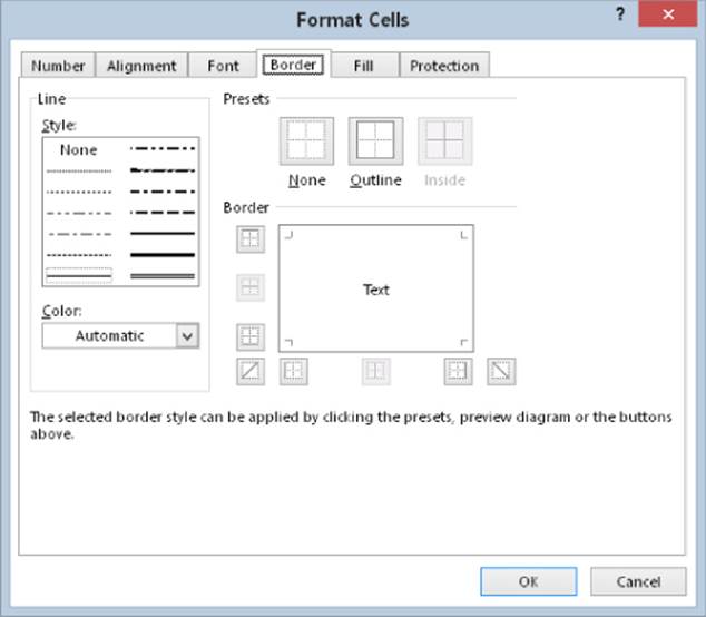
Figure 6.10 Use the Border tab of the Format Cells dialog box for more control over cell borders.

Before you display the Format Cells dialog box, select the cell or range to which you want to add borders. First choose a line style, and then choose the border position for the line style by clicking one of the Border icons. (These icons are toggles.)

Notice that the Border tab has three preset icons, which can save you some clicking. If you want to remove all borders from the selection, click None. To put an outline around the selection, click Outline. To put borders inside the selection, click Inside.

Excel displays the selected border style in the dialog box; there is no live preview. You can choose different styles for different border positions; you can also choose a color for the border. Using this dialog box may require some experimentation, but you'll get the hang of it.

When you apply two diagonal lines, the cells look like they've been crossed out.

Tip

If you use border formatting in your worksheet, you may want to turn off the grid display to make the borders more pronounced. Choose View Show Gridlines to toggle the gridline display.

Adding a Background Image to a Worksheet

In some situations, you might want to use a graphics file to serve as a background for a worksheet. This effect is similar to the wallpaper that you may display on your Windows desktop or as a background for a web page.

To add a background to a worksheet, choose Page Layout Page Setup Background. Excel displays a dialog box that enables you to select a graphics file. All common graphics file formats are supported, but animated GIFs display as static images. When you locate a file, click Insert. Excel tiles the graphic across your worksheet. Some images are specifically designed to be tiled, such as the one shown in Figure 6.11. This type of image is often used for web pages, and it creates a seamless background.

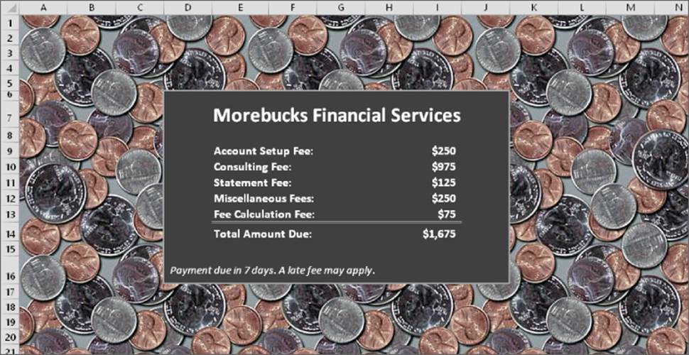
Figure 6.11 You can add almost any image file as a worksheet background image.

This workbook, named background image.xlsx, is available on this book's website at www.wiley.com/go/excel2016bible.

When you use a background image, you'll probably want to turn off the gridline display because the gridlines show through the graphic. Some backgrounds make viewing text difficult, so you may want to use a solid background color for cells that contain text.

Keep in mind that using a background image will increase the size of your workbook because the image is stored in the workbook file.

Note

The graphics background on a worksheet is for onscreen display only — it isn't printed when you print the worksheet.

Copying Formats by Painting

Perhaps the quickest way to copy the formats from one cell to another cell or range is to use the Format Painter button (the button with the paintbrush image) of the Home Clipboard group.

1. Select the cell or range that has the formatting attributes you want to copy.

2. Click the Format Painter button. The mouse pointer changes to include a paintbrush.

3. Select the cells to which you want to apply the formats.

4. Release the mouse button, and Excel applies the same set of formatting options that were in the original range.

If you double-click the Format Painter button, you can paint multiple areas of the worksheet with the same formats. Excel applies the formats that you copy to each cell or range that you select. To get out of Paint mode, click the Format Painter button again (or press Esc).

Using Named Styles for Easier Formatting

One of the most underutilized features in Excel is named styles. Named styles make it easy to apply a set of predefined formatting options to a cell or range. In addition to saving time, using named styles helps to ensure a consistent look.

A style can consist of settings for up to six attributes:

· Number format

· Alignment (vertical and horizontal)

· Font (type, size, and color)

· Borders

· Fill

· Cell protection (locked and hidden)

The real power of styles is apparent when you change a component of a style. All cells that use that named style automatically incorporate the change. Suppose that you apply a particular style to a dozen cells scattered throughout your worksheet. Later, you realize that these cells should have a font size of 14 pt rather than 12 pt. Rather than change each cell, simply edit the style. All cells with that particular style change automatically.

Applying styles

Excel includes a good selection of predefined named styles that work in conjunction with document themes. Figure 6.12 shows the effect of choosing Home Styles Cell Styles. Note that this display is a live preview — as you move your mouse over the style choices, the selected cell or range temporarily displays the style. When you see a style you like, click it to apply the style to the selection.

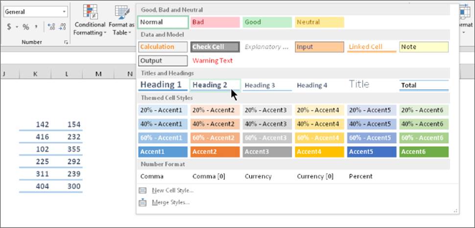
Figure 6.12 Excel displays samples of predefined cell styles.

Note

If Excel's window is wide enough, you won't see the Cell Styles command in the Ribbon. Instead, you'll see four or more formatted style boxes. Click the drop-down arrow to the right of these boxes to display all the defined styles.

Note

By default, all cells use the Normal style. If you modify the Normal style, all cells that haven't been assigned a different style will reflect the new formatting.

After you apply a style to a cell, you can apply additional formatting to it by using any formatting method discussed in this chapter. Formatting modifications that you make to the cell don't affect other cells that use the same style.

You have quite a bit of control over styles. In fact, you can do any of the following:

· Modify an existing style.

· Create a new style.

· Merge styles from another workbook into the active workbook.

The following sections describe these procedures.

Modifying an existing style

To change an existing style, choose Home Styles Cell Styles. Right-click the style you want to modify and choose Modify from the shortcut menu. Excel displays the Style dialog box, shown in Figure 6.13. In this example, the Style dialog box shows the settings for the Office theme Normal style — which is the default style for all cells. The style definitions vary, depending on which document theme is active.

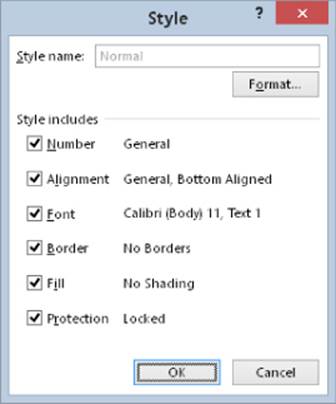
Figure 6.13 Use the Style dialog box to modify named styles.

Here's a quick example of how you can use styles to change the default font used throughout your workbook:

1. Choose Home Styles Cell Styles. Excels displays the list of styles for the active workbook.

2. Right-click Normal and choose Modify. Excel displays the Style dialog box (refer to Figure 6.13), with the current settings for the Normal style.

3. Click the Format button. Excel displays the Format Cells dialog box.

4. Click the Font tab and choose the font and size that you want as the default.

5. Click OK to return to the Style dialog box. Notice that the Font item displays the font choice you made.

6. Click OK again to close the Style dialog box.

The font for all cells that use the Normal style changes to the font that you specified. You can change any formatting attributes for any style.

Creating new styles

In addition to using Excel's built-in styles, you can create your own styles. This feature can be quite handy because it enables you to apply your favorite formatting options quickly and consistently.

To create a new style, follow these steps:

1. Select a cell and apply all the formatting that you want to include in the new style. You can use any of the formatting that is available in the Format Cells dialog box (refer to Figures 6.3 and 6.5).

2. After you format the cell to your liking, choose Home Styles Cell Styles, and choose New Cell Style. Excel displays its Style dialog box (refer to Figure 6.13), along with a proposed generic name for the style. Note that Excel displays the wordsBy Example to indicate that it's basing the style on the current cell.

3. Enter a new style name in the Style Name field. The check boxes display the current formats for the cell. By default, all check boxes are selected.

4. (Optional) If you don't want the style to include one or more format categories, remove the check(s) from the appropriate check box(es).

5. Click OK to create the style and to close the dialog box.

After you perform these steps, the new custom style is available when you choose Home Styles Cell Styles. Custom styles are available only in the workbook in which they were created. To copy your custom styles to another workbook, see the section that follows.

Note

The Protection option in the Style dialog box controls whether users will be able to modify cells for the selected style. This option is effective only if you've also turned on worksheet protection by choosing Review Changes Protect Sheet.

Merging styles from other workbooks

Custom styles are stored with the workbook in which they were created. If you've created some custom styles, you probably don't want to go through all the work to create copies of those styles in each new Excel workbook. A better approach is to merge the styles from a workbook in which you previously created them.

To merge styles from another workbook, open both the workbook that contains the styles that you want to merge and the workbook that will contain the merged styles. Activate the second workbook, choose Home Styles Cell Styles, and then choose Merge Styles. Excel displays the Merge Styles dialog box that shows a list of all open workbooks. Select the workbook that contains the styles you want to merge and click OK. Excel copies styles from the workbook that you selected into the active workbook.

Controlling styles with templates

When you start Excel, it loads with several default settings, including the settings for stylistic formatting. If you spend a lot of time changing the default elements for every new workbook, you should know about templates.

Here's an example. You may prefer that gridlines aren't displayed in worksheets. And maybe you prefer Wrap Text to be the default setting for alignment. Templates provide an easy way to change defaults.

The trick is to create a workbook with the Normal style modified in the way that you want it. Then save the workbook as a template (with an .xltx extension). After doing so, you can choose this template as the basis for a new workbook.

Refer to Chapter 8, “Using and Creating Templates,” for more information about templates.

Understanding Document Themes

In an attempt to help users create more professional-looking documents, the Office designers incorporated a feature known as document themes. Using themes is an easy (and almost foolproof) way to specify the colors, fonts, and a variety of graphic effects in a document. And best of all, changing the entire look of your document is a breeze. A few mouse clicks is all it takes to apply a different theme and change the look of your workbook.

Importantly, the concept of themes is incorporated into other Office applications. Therefore, a company can easily create a standard and consistent look for all its documents.

Note

Themes don't override specific formatting that you apply. For example, assume that you apply the Accent 1 named style to a range. Then you change the font color for a few cells in that range. If you change to a different theme, the manually applied fonts won't be modified to use the new theme fonts. Bottom line: if you plan to take advantage of themes, stick with default formatting choices.

Figure 6.14 shows a worksheet that contains a SmartArt diagram, a table, a chart, a range formatted with the Title named style, and a range formatted with the Explanatory Text named style. These items all use the default theme, which is the Office Theme.

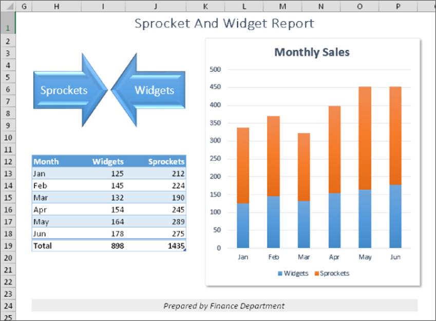
Figure 6.14 The elements in this worksheet use the default theme.

Figure 6.15 shows the same worksheet after applying a different document theme. The different theme changed the fonts, colors (which may not be apparent in the figure), and the graphics effects for the SmartArt diagram.

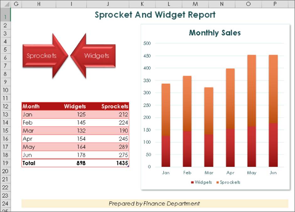
Figure 6.15 The worksheet after applying a different theme.

If you'd like to experiment with using various themes, the workbook shown in Figure 6.14 and Figure 6.15 is available on this book's website at www.wiley.com/go/excel2016bible. The file is named theme examples.xlsx.

Applying a theme

Figure 6.16 shows the theme choices that appear when you choose Page Layout Themes Themes. This display is a live preview. As you move your mouse over the theme choices, the active worksheet displays the theme. When you see a theme you like, click it to apply the theme to all worksheets in the workbook.

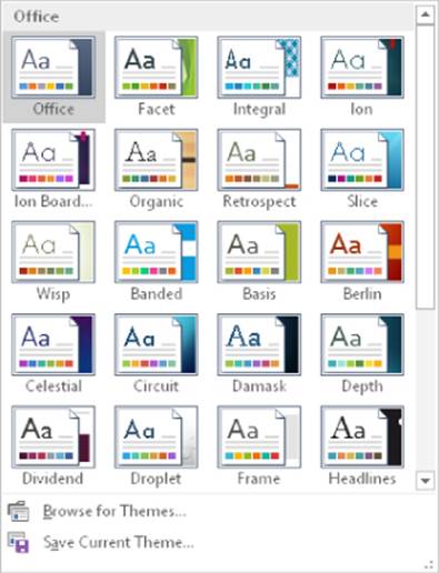
Figure 6.16 Built-in Excel theme choices.

Note

A theme applies to the entire workbook. You can't use different themes on different worksheets within a workbook.

When you specify a particular theme, the gallery choices for various elements reflect the new theme. For example, the chart styles that you can choose from vary, depending on which theme is active.

Note

Because themes use different fonts (which can vary in size), changing to a different theme may affect the layout of your worksheet. For example, after you apply a new theme, a worksheet that printed on a single page may spill over to a second page. Therefore, you may need to make some adjustments after you apply a new theme.

Customizing a theme

Notice that the Themes group on the Page Layout tab contains three other controls: Colors, Fonts, and Effects. You can use these controls to change just one of the three components of a theme. For example, you might like the colors and effects in the Office theme but would prefer different fonts. To change the font set, apply the Office theme and then specify your preferred font set by choosing Page Layout Themes Font.

Each theme uses two fonts (one for headers, and one for the body), and in some cases, these two fonts are the same. If none of the theme choices is suitable, choose Page Layout Themes Font Customize Fonts to specify the two fonts you prefer (see Figure 6.17).

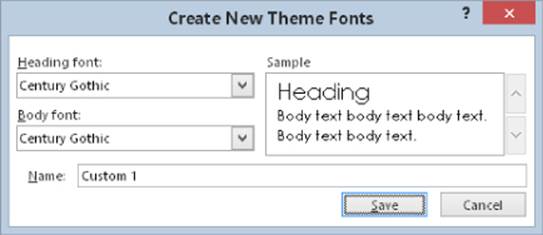
Figure 6.17 Use this dialog box to specify two fonts for a theme.

Tip

When you choose Home Font Font, the two fonts for the current theme are listed first in the drop-down list.

Choose Page Layout Themes Colors to select a different set of colors. And, if you're so inclined, you can even create a custom set of colors by choosing Page Layout Themes Colors Customize Colors. This command displays the Create New Theme Colors dialog box, shown in Figure 6.18. Note that each theme consists of twelve colors. Four of the colors are for text and backgrounds, six are for accents, and two are for hyperlinks. As you specify different colors, the preview panel in the dialog box updates.

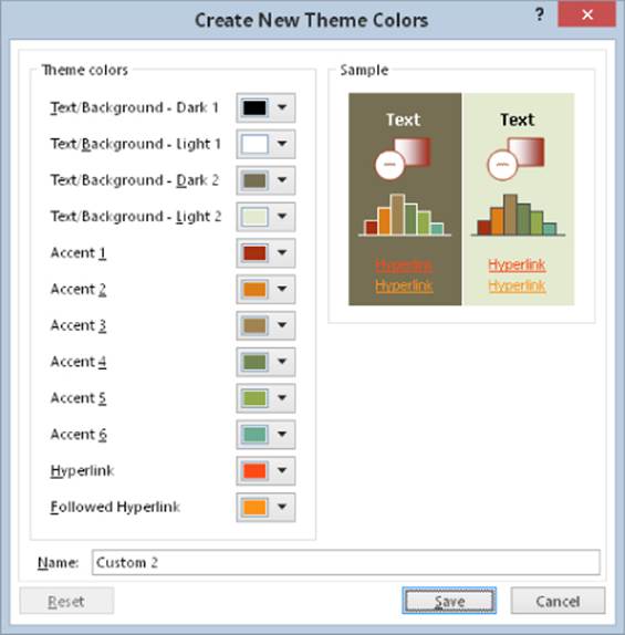
Figure 6.18 If you're feeling creative, you can specify a set of custom colors for a theme.

Note

Theme effects operate on graphics elements, such as SmartArt, Shapes, and charts. You can choose a different set of theme effects, but you can't customize theme effects.

If you've customized a theme using different fonts or colors, you can save the new theme by choosing Page Layout Themes Save Current Theme. Your customized themes appear in the theme list in the Custom category. Other Office applications, such as Word and PowerPoint, can use these theme files.