Microsoft Excel 2016 BIBLE (2016)

IN THIS CHAPTER

1. Changing your worksheet view

2. Adjusting your print settings for better results

3. Preventing some cells from being printed

4. Using the Custom Views feature

5. Creating PDF files

Despite predictions of the “paperless office,” reports printed on paper remain commonplace, and office printers will be around for a long time. Many worksheets that you develop with Excel will eventually end up as hard-copy reports. You'll find that printing from Excel is quite easy and that you can generate attractive, well-formatted reports with minimal effort. In addition, Excel has many options that give you a great deal of control over the printed page. These options are explained in this chapter.

Basic Printing

If you want to print a copy of a worksheet with no fuss and bother, use the Quick Print option. One way to access this command is to choose File Print (which displays the Print pane of Backstage view) and then click the Print button.

If you like the idea of one-click printing, take a few seconds to add a new button to your Quick Access toolbar. Click the downward-pointing arrow on the right of the Quick Access toolbar and then choose Quick Print from the drop-down list. Excel adds the Quick Print icon to your Quick Access toolbar.

Clicking the Quick Print button prints the current worksheet on the currently selected printer, using the default print settings. If you've changed any of the default print settings (by using the Page Layout tab), Excel uses the new settings; otherwise, it uses the following default settings:

· Prints the active worksheet (or all selected worksheets), including any embedded charts or objects

· Prints one copy

· Prints the entire active worksheet

· Prints in portrait mode

· Doesn't scale the printed output

· Uses letter-size paper with 0.75-inch margins for the top and bottom and 0.70-inch margins for the left and right margins (for the U.S. version)

· Prints with no headers or footers

· Doesn't print cell comments

· Prints with no cell gridlines

· For wide worksheets that span multiple pages, prints down and then over

When you print a worksheet, Excel prints only the active area of the worksheet. In other words, it won't print all 17 billion cells — just those that have data in them. If the worksheet contains any embedded charts or other graphic objects (such as SmartArt or Shapes), they're also printed.

Using Print Preview

When you choose File Print (or press Ctrl+P), Backstage view displays a preview of your printed output, exactly as it will be printed. Initially, Excel displays the first page of your printed output. To view subsequent pages, use the page controls along the bottom of the preview pane (or use the vertical scrollbar along the right side of the screen).

The Print Preview window has a few other commands (at the bottom) that you can use while previewing your output. For multipage printout, use the page number controls to quickly jump to a particular page. The Show Margins button toggles the display of margins, and Zoom to Page ensures that a complete page is displayed.

When the Show Margins option is in effect, Excel adds markers to the preview that indicate column borders and margins. You can drag the column or margin markers to make changes that appear onscreen. Changes that you make to column widths in preview mode are also made in the actual worksheet.

Print Preview is certainly useful, but you may prefer to use Page Layout view to preview your output (see “Changing Your Page View”).

Changing Your Page View

Page Layout view shows your worksheet divided into pages. In other words, you can visualize your printed output while you work.

Page Layout view is one of three worksheet views, which are controlled by the three icons on the right side of the status bar. You could also use the commands in the View Workbook Views group on the Ribbon to switch views. The three view options are

· Normal: The default view of the worksheet. This view may or may not show page breaks.

· Page Layout: Shows individual pages.

· Page Break Preview: Allows you to manually adjust page breaks.

Just click one of the icons to change the view. You can also use the Zoom slider to change the magnification from 10% (a very tiny, bird's-eye view) to 400% (very large, for showing fine detail).

The following sections describe how these views can help with printing.

Normal view

Most of the time when you work in Excel, you use Normal view. Normal view can display page breaks in the worksheet. The page breaks are indicated by horizontal and vertical ­dotted lines. These page break lines adjust automatically if you change the page orientation, add or delete rows or columns, change row heights, change column widths, and so on. For example, if you find that your printed output is too wide to fit on a single page, you can adjust the column widths (keeping an eye on the page break display) until the columns are narrow enough to print on one page.

Note

Page breaks aren't displayed until you print (or preview) the worksheet at least one time. Page breaks are also displayed if you set a print area by choosing Page Layout Page Setup Print Area.

Tip

If you'd prefer not to see the page break display in Normal view, choose File Options and select the Advanced tab. Scroll down to the Display Options for This Worksheet section and remove the check mark from Show Page Breaks. This setting applies only to the active worksheet. Unfortunately, the option to turn off page break display is not on the Ribbon, and it's not even available for inclusion on the Quick Access toolbar. This is another one of those little annoyances that I expect Microsoft to fix one of these times.

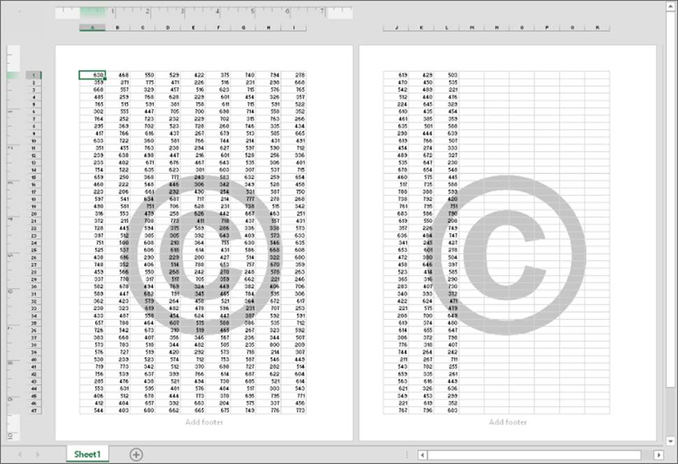
Figure 9.1 shows a worksheet in Normal view, zoomed out to show multiple pages. Notice the dotted lines that indicate page breaks.

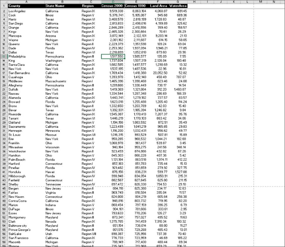
Figure 9.1 In Normal view, dotted lines indicate page breaks.

Page Layout view

Page Layout view is the ultimate print preview. Unlike the preview in Backstage view (choose File Print), this mode is not a view-only mode. You have complete access to all Excel commands. In fact, you can use Page Layout view all the time if you like.

Figure 9.2 shows a worksheet in Page Layout view, zoomed out to show multiple pages. Notice that the page header and footer (if any) appear on each page. If you've specified any repeated rows and columns, they also display — giving you a true preview of the printed output.

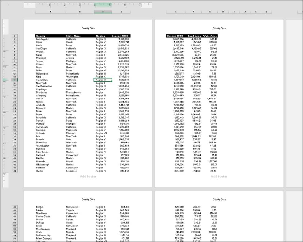
Figure 9.2 In Page Layout view, the worksheet resembles printed pages.

Tip

If you move the mouse to the corner of a page while in Page Layout view, you can click to hide the white space in the margins. Doing so gives you all the advantages of Page Layout view, but you can see more information onscreen because the unused margin space is hidden.

Page Break Preview

Page Break Preview displays the worksheet and the page breaks. Figure 9.3 shows an example. This view mode is different from Normal view mode with page breaks turned on. The key difference is that you can drag the page breaks. Unlike Page Layout view, Page Break Preview does not display headers and footers.

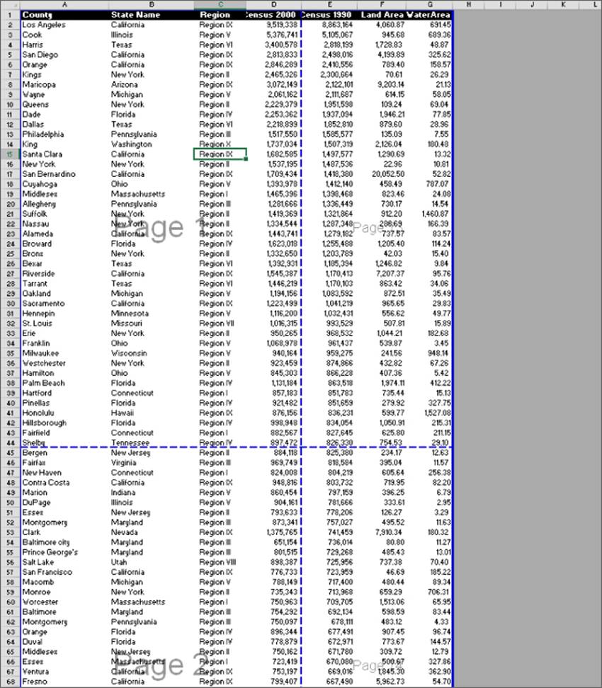
Figure 9.3 Page Break Preview mode gives you a bird's-eye view of your worksheet and shows exactly where the page breaks occur.

When you enter Page Break Preview, Excel performs the following:

· Changes the zoom factor so that you can see more of the worksheet.

· Displays the page numbers overlaid on the pages.

· Displays the current print range with a white background; nonprinting data appears with a gray background.

· Displays all page breaks as draggable dashed lines.

When you change the page breaks by dragging, Excel automatically adjusts the scaling so that the information fits on the pages, per your specifications.

Tip

In Page Break Preview, you still have access to all Excel commands. You can change the zoom factor if you find the text to be too small.

To exit Page Break Preview, just click one of the other View icons on the right side of the status bar.

Adjusting Common Page Setup Settings

Clicking the Quick Print button (or choosing File Print Print) may produce acceptable results in many cases, but a little tweaking of the print settings can often improve your printed reports. You can adjust print settings in three places:

· The Print settings screen in Backstage view, displayed when you choose File Print.

· The Page Layout tab of the Ribbon.

· The Page Setup dialog box, displayed when you click the dialog launcher in the lower-right corner of the Page Layout Page Setup group on the Ribbon. You can also access the Page Setup dialog box from the Print settings screen in Backstage view.

Table 9.1 summarizes the locations where you can make various types of print-related adjustments in Excel 2016.

Table 9.1 Where to Change Printer Settings

Table 9.1 might make printing seem more complicated than it really is. The key point to remember is this: if you can't find a way to make a particular adjustment, it's probably available from the Page Setup dialog box.

Choosing your printer

To switch to a different printer or output device, choose File Print, and use the drop-down control in the Printer section to select a different installed printer.

Note

To adjust printer settings, click the Printer Properties link to display a property box for the selected printer. The exact dialog box that you see depends on the printer. The Properties dialog box lets you adjust printer-specific settings, such as the print quality and the paper source. In most cases, you won't have to change any of these settings, but if you're having print-related problems, you may want to check the settings.

Specifying what you want to print

Sometimes you may want to print only a part of the worksheet rather than the entire active area. Or you may want to reprint selected pages of a report without printing all the pages. Choose File Print, and use the controls in the Settings section to specify what to print.

You have several options:

· Print Active Sheets: Prints the active sheet or sheets that you selected. (This option is the default.) You can select multiple sheets to print by pressing Ctrl and clicking the sheet tabs. If you select multiple sheets, Excel begins printing each sheet on a new page.

· Print Entire Workbook: Prints the entire workbook, including chart sheets.

· Print Selection: Prints only the range that you selected before choosing File Print.

· Print Selected Chart: Appears only if a chart is selected. If this option is chosen, only the chart will be printed.

· Print Selected Table: Appears only if the cell pointer is within a table (created by choosing Insert Tables Table) when the Print Setting screen is displayed. If this option is chosen, only the table will be printed.

Tip

You can also choose Page Layout Page Setup Print Area Set Print Area to specify the range(s) to print. Before you choose this command, select the range(s) that you want to print. To clear the print area, choose Page Layout Page Setup Print Area Clear Print Area. To override the print area, select the Ignore Print Area check box in the list of Print What options.

Note

The print area does not have to be a single range. You make a multiple selection before you set the print area. Each area will print on a separate page.

If your printed output uses multiple pages, you can select which pages to print by indicating the number of the first and last pages to print by using Pages controls in the Settings section. You can either use the spinner controls or type the page numbers in the edit boxes.

Changing page orientation

Page orientation refers to the way output is printed on the page. Choose Page Layout Page Setup Orientation Portrait to print tall pages (the default) or Page Layout Page Setup Orientation Landscape to print wide pages. Landscape orientation is useful when you have a wide range that doesn't fit on a vertically oriented page.

If you change the orientation, the onscreen page breaks adjust automatically to accommodate the new paper orientation.

Page orientation settings are also available when you choose File Print.

Specifying paper size

Choose Page Layout Page Setup Size to specify the paper size you're using. The paper size settings are also available when you choose File Print.

Note

Even though Excel displays a variety of paper sizes, your printer may not be capable of using all of them.

Printing multiple copies of a report

Use the Copies control at the top of the Print tab in Backstage View to specify the number of copies to print. Just enter the number of copies you want and then click Print.

Tip

If you're printing multiple copies of a report, make sure that the Collated option is selected so that Excel prints the pages in order for each set of output. If you're printing only one page, Excel ignores the Collated setting.

Adjusting the page margins

Margins are the unprinted areas along the sides, top, and bottom of a printed page. Excel provides four “quick margin” settings; you can also specify the exact margin size you require. All printed pages have the same margins. You can't specify different margins for different pages.

In Page Layout view, a ruler is displayed above the column header and to the left of the row header. Use your mouse to drag the margins in the ruler. Excel adjusts the page display immediately. Use the horizontal ruler to adjust the left and right margins, and use the vertical ruler to adjust the top and bottom margins.

From the Page Layout Page Setup Margins drop-down list, you can select Normal, Wide, Narrow, or the Last Custom Setting. These options are also available when you choose File Print. If none of these settings does the job, choose Custom Margins to display the Margins tab of the Page Setup dialog box, shown in Figure 9.4.

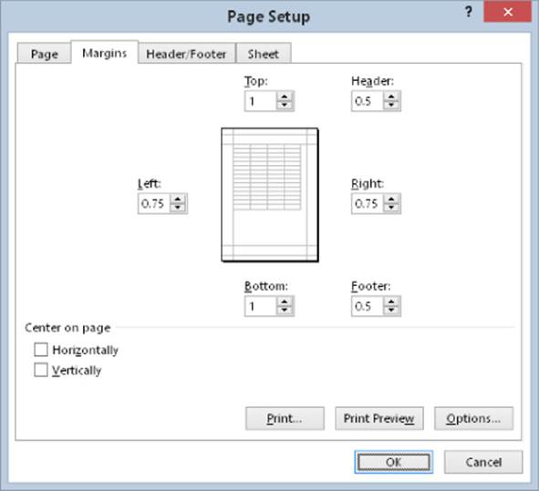
Figure 9.4 The Margins tab of the Page Setup dialog box.

To change a margin, click the appropriate spinner (or you can enter a value directly). The margin settings that you specify in the Page Setup dialog box will then be available in the Page Layout Page Setup Margins drop-down list, referred to as Last Custom Setting.

Note

The Preview box in the center of the Page Setup dialog box is a bit deceiving because it doesn't really show you how your changes look in relation to the page; instead, it displays a darker line to let you know which margin you're adjusting.

You can also adjust margins in the preview window in Backstage view (choose File Print). Click the Show Margins button in the bottom-right corner to display the margins in the preview pane. Then drag the margin indicators to adjust the margins.

In addition to the page margins, you can adjust the distance of the header from the top of the page and the distance of the footer from the bottom of the page. These settings should be less than the corresponding margin; otherwise, the header or footer may overlap with the printed output.

By default, Excel aligns the printed page at the top and left margins. If you want the output to be centered vertically or horizontally, select the appropriate check box in the Center on Page section of the Margins tab.

Understanding page breaks

When printing lengthy reports, controlling where pages break is often important. For example, you probably don't want a row to print on a page by itself, nor do you want a table header row to be the last line on a page. Fortunately, Excel gives you precise control over page breaks.

Excel handles page breaks automatically, but sometimes you may want to force a page break — either a vertical or a horizontal one — so that the report prints the way you want. For example, if your worksheet consists of several distinct sections, you may want to print each section on a separate sheet of paper.

Inserting a page break

To insert a horizontal page break line, move the cell pointer to the cell that will begin the new page. Make sure that you place the pointer in column A, though; otherwise, you'll insert a vertical page break and a horizontal page break. For example, if you want row 14 to be the first row of a new page, select cell A14. Then choose Page Layout Page Setup Breaks Insert Page Break.

Note

Page breaks are visualized differently, depending on which view mode you're using. (See “Changing Your Page View,” earlier in this chapter.)

To insert a vertical page break line, move the cell pointer to the cell that will begin the new page. In this case, though, make sure to place the pointer in row 1. Choose Page Layout Page Setup Breaks Insert Page Break to create the page break.

Removing manual page breaks

To remove a page break you've added, move the cell pointer to the first row beneath (or the first column to the right of) the manual page break and then choose Page Layout Page Setup Breaks Remove Page Break.

To remove all manual page breaks in the worksheet, choose Page Layout Page Setup Breaks Reset All Page Breaks.

Printing row and column titles

If your worksheet is set up with titles in the first row and descriptive names in the first column, it can be difficult to identify data that appears on printed pages where those titles don't appear. To resolve this problem, you can choose to print selected rows or columns as titles on each page of the printout.

Row and column titles serve pretty much the same purpose on a printout as frozen panes do in navigating within a worksheet. Keep in mind, however, that these features are independent of each other. In other words, freezing panes doesn't affect the printed output.

See Chapter 3, “Essential Worksheet Operations,” for more information on freezing panes.

Caution

Don't confuse print titles with headers; these are two different concepts. Headers appear at the top of each page and contain information, such as the worksheet name, date, or page number. Row and column titles describe the data being printed, such as field names in a database table or list.

You can specify particular rows to repeat at the top of every printed page or particular columns to repeat at the left of every printed page. To do so, choose Page Layout Page Setup Print Titles. Excel displays the Sheet tab of the Page Setup dialog box, shown inFigure 9.5.

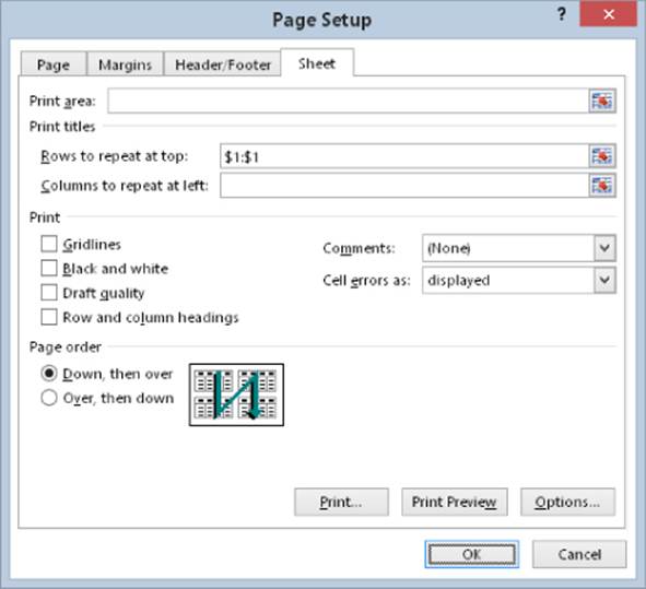
Figure 9.5 Use the Sheet tab of the Page Setup dialog box to specify rows or columns that will appear on each printed page.

Activate the appropriate box (either Rows to Repeat at Top or Columns to Repeat at Left) and then select the rows or columns in the worksheet. Or you can enter these references manually. For example, to specify rows 1 and 2 as repeating rows, enter 1:2.

Note

When you specify row and column titles and use Page Layout view, these titles will repeat on every page (just as when the document is printed). However, the cells used in the title can be selected only on the page in which they first appear.

Scaling printed output

In some cases, you may need to force your printed output to fit on a specific number of pages. You can do so by enlarging or reducing the size. To enter a scaling factor, choose Page Layout Scale to Fit Scale. You can scale the output from 10% up to 400%. To return to normal scaling, enter 100%.

To force Excel to print using a specific number of pages, choose Page Layout Scale to Fit Width and Page Layout Scale to Fit Height. When you change either one of these settings, the corresponding scale factor is displayed in the Scale control.

Caution

Excel doesn't ensure legibility. It will gladly scale your output to be so small that no one can read it.

Printing cell gridlines

Typically, cell gridlines aren't printed. If you want your printout to include the gridlines, choose Page Layout Sheet Options Gridlines Print.

Alternatively, you can insert borders around some cells to simulate gridlines.

See Chapter 6, “Worksheet Formatting,” for information about borders.

Printing row and column headers

By default, row and column headers for a worksheet are not printed. If you want your printout to include these items, choose Page Layout Sheet Options Headings Print.

Using a background image

Would you like to have a background image on your printouts? Unfortunately, you can't. You may have noticed the Page Layout Page Setup Background command. This button displays a dialog box that lets you select an image to display as a background. Placing this control among the other print-related commands is misleading. Background images placed on a worksheet are never printed.

Tip

In lieu of a true background image, you can insert WordArt, a Shape, or a picture on your worksheet and then adjust its transparency. Then copy the image to all printed pages. Alternatively, you can insert an object in a page header or footer. (See the next sidebar, “Inserting a Watermark.”)

Inserting a Watermark

A watermark is an image (or text) that appears on each printed page. A watermark can be a faint company logo or a word such as DRAFT. Excel doesn't have an official command to print a watermark, but you can add a watermark by inserting a picture in the page header or footer. Here's how:

1. Locate an image on your hard drive that you want to use for the watermark.

2. Choose View Workbook Views Page Layout View.

3. Click the center section of the header.

4. Choose Header & Footer Tools Design Header & Footer Elements Picture. The Insert Pictures dialog box appears.

5. Click Browse and locate the image from step 1 (or locate a suitable image from other sources listed).

6. Click outside the header to see your image.

7. To center the image in the middle of the page, click the center section of the header and add some carriage returns before the &[Picture] code. You'll need to experiment to determine the number of carriage returns required to push the image into the body of the document.

8. If you need to adjust the image (for example, make it lighter), click the center section of the header and then choose Header & Footer Tools Design Header & Footer Elements Format Picture. Use the Image controls in the Picture tab of the Format Picture dialog box to adjust the image. You may need to experiment with the settings to make sure that the worksheet text is legible.

The accompanying figure shows an example of a header image (a copyright symbol) used as a watermark. You can do a similar thing with text, of course.

Adding a Header or a Footer to Your Reports

A header is information that appears at the top of each printed page. A footer is information that appears at the bottom of each printed page. By default, new workbooks do not have headers or footers.

You can specify headers and footers by using the Header/Footer tab of the Page Setup dialog box. Or simplify the task by switching to Page Layout view, where you can click the section labeled Click to Add Header or Click to Add Footer.

Note

If you're working in Normal view, you can choose Insert Text Header & Footer. Excel switches to Page Layout view and activates the center section of the page header.

You can then type the information and apply any type of formatting you like. Note that headers and footers consist of three sections: left, center, and right. For example, you can create a header that prints your name at the left margin, the worksheet name centered in the header, and the page number at the right margin.

Tip

If you want a consistent header or footer for all your documents, create a book.xltx template with your headers or footers specified. A book.xltx template is used as the basis for new workbooks.

See Chapter 8, “Using and Creating Templates,” for details on creating a template.

When you activate the header or footer section in Page Layout view, the Ribbon displays a new contextual tab: Header & Footer Tools Design. Use the controls on this tab to work with headers and footers.

Selecting a predefined header or footer

You can choose from a number of predefined headers or footers by using either of the two drop-down lists in the Header & Footer Tools Design Header & Footer group. Notice that some items in these lists consist of multiple parts, separated by a comma. Each part goes into one of the three header or footer sections (left, center, or right). Figure 9.6 shows an example of a header that uses all three sections.

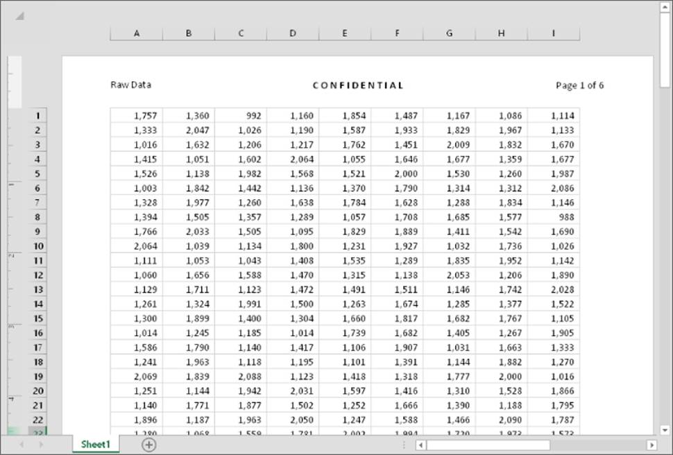
Figure 9.6 This three-part header is one of Excel's predefined headers.

Understanding header and footer element codes

When a header or footer section is activated, you can type whatever text you like into the section. Or to insert variable information, you can insert any of several element codes by clicking a button in the Header & Footer Tools Design Header & Footer Elements group. Each button inserts a code into the selected section. For example, to insert the current date, click the Current Date button. Table 9.2 lists the buttons and their functions.

Table 9.2 Header and Footer Buttons and Their Functions

You can combine text and codes and insert as many codes as you like into each section.

Note

If the text that you enter uses an ampersand (&), you must enter the ampersand twice (because Excel uses an ampersand to signal a code). For example, to enter the text Research & Development into a section of a header or footer, type Research && Development.

You can also use different fonts and sizes in your headers and footers. Just select the text that you want to change and then use the formatting tools in the Home Font group. Or use the controls on the Mini toolbar, which appears automatically when you select the text. If you don't change the font, Excel uses the font defined for the Normal style.

Tip

You can use as many lines as you like. Press Enter to force a line break for multiline headers or footers. If you use multiline headers or footers, you may need to adjust the top or bottom margin so the text won't overlap with the worksheet data. (See “Adjusting the page margins,” earlier in this chapter.)

Unfortunately, you can't print the contents of a specific cell in a header or footer. For example, you may want Excel to use the contents of cell A1 as part of a header. To do so, you need to enter the cell's contents manually — or write a VBA macro to perform this operation before the sheet is printed.

Other header and footer options

When a header or footer is selected in Page Layout view, the Header & Footer Design Options group contains controls that let you specify other options:

· Different First Page: If checked, you can specify a different header/footer for the first printed page.

· Different Odd & Even Pages: If checked, you can specify a different header/footer for odd and even pages.

· Scale with Document: If checked, the font size in the header and footer will be sized accordingly if the document is scaled when printed. This option is enabled by default.

· Align with Page Margins: If checked, the left header and footer will be aligned with the left margin, and the right header and footer will be aligned with the right margin. This option is enabled by default.

Other Print-Related Topics

The following sections cover some additional topics related to printing from Excel.

Copying Page Setup settings across Sheets

Each Excel worksheet has its own print setup options (orientation, margins, headers and footers, and so on). These options are specified in the Page Setup group of the Page Layout tab.

When you add a new sheet to a workbook, it contains the default page setup settings. Here's an easy way to transfer the settings from one worksheet to additional worksheets:

1. Activate the sheet that contains the desired setup information. This is the source sheet.

2. Select the target sheets. Ctrl+click the sheet tabs of the sheets you want to update with the settings from the source sheet.

3. Click the dialog box launcher in the lower-right corner of the Page Layout Page Setup group.

4. When the Page Setup dialog box appears, click OK to close it.

5. Ungroup the sheets by right-clicking any selected sheet and choosing Ungroup Sheets from the shortcut menu. Because multiple sheets are selected when you close the Page Setup dialog box, the settings of the source sheet will be transferred to all target sheets.

Note

Two settings located on the Sheet tab of the Page Setup dialog box are not transferred: Print Area and Print Titles. In addition, pictures in the header or footer are not transferred.

Preventing certain cells from being printed

If your worksheet contains confidential information, you may want to print the worksheet but not the confidential parts. You can use several techniques to prevent certain parts of a worksheet from printing:

· Hide rows or columns. When you hide rows or columns, the hidden rows or columns aren't printed. Choose Home Cells Format drop-down list to hide the selected rows or columns.

· Hide cells or ranges.

· You can hide cells or ranges by making the text color the same color as the background color. Be aware, however, that this method may not work for all printers.

· You can hide cells by using a custom number format that consists of three semicolons (;;;). See Chapter 25, “Using Custom Number Formats,” for more information about using custom number formats.

· Mask an area. You can mask a confidential area of a worksheet by covering it with a rectangle Shape. Choose Insert Illustrations Shapes and click the Rectangle Shape. You'll probably want to adjust the fill color to match the cell background and remove the border.

If you find that you must regularly hide data before you print certain reports, consider using the Custom Views feature, discussed later in this chapter. (See “Creating custom views of your worksheet.”) This feature allows you to create a named view that doesn't show the confidential information.

Preventing objects from being printed

To prevent objects on the worksheet (such as charts, Shapes, and SmartArt) from being printed, you need to access the Properties tab of the object's Format dialog box (see Figure 9.7):

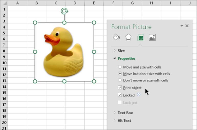
Figure 9.7 Use the Properties tab of the object's Format dialog box to prevent objects from printing.

1. Right-click the object and choose Format xxxx from the shortcut menu. (xxxx varies, depending on the object.)

2. In the Format dialog box that opens for the object, click the Size & Properties icon.

3. Expand the Properties section of the dialog box.

4. Remove the check mark for Print Object.

Note

For a chart, you must right-click the chart's Chart Area (the background of the chart). Or double-click the chart's border to display the Format Chart Area dialog box. Then expand the Properties section and remove the check mark from Print Object.

Creating custom views of your worksheet

If you need to create several different printed reports from the same Excel workbook, setting up the specific settings for each report can be a tedious job. For example, you may need to print a full report in landscape mode for your boss. Another department may require a simplified report using the same data, but with some hidden columns in portrait mode. You can simplify the process by creating custom named views of your worksheets that include the proper settings for each report.

The Custom Views feature enables you to give names to various views of your worksheet. You can quickly switch among these named views. A view includes settings for the following:

· Print settings, as specified in the Page Layout Page Setup, Page Layout Scale to Fit, and Page Page Setup Sheet Options groups

· Hidden rows and columns

· The worksheet view (Normal, Page Layout, Page Break preview)

· Selected cells and ranges

· The active cell

· The zoom factor

· Window sizes and positions

· Frozen panes

If you find that you're constantly fiddling with these settings before printing and then changing them back, using named views can save you some work.

Caution

Unfortunately, the Custom Views feature doesn't work if the workbook (not just the worksheet) contains at least one table — created using Insert Tables Table. When a workbook that contains a table is active, the Custom View command is disabled. This limitation severely limits the usefulness of the Custom Views feature.

To create a named view, follow these steps:

1. Set up the view settings the way you want them. For example, hide some columns.

2. Choose View Workbook Views Custom Views. The Custom Views dialog box appears.

3. Click the Add button. The Add View dialog box (shown in Figure 9.8) appears.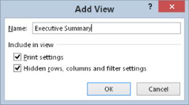

Figure 9.8 Use the Add View dialog box to create a named view.

4. Provide a descriptive name. You can also specify what to include in the view by using the two check boxes. For example, if you don't want the view to include print settings, remove the check mark from Print Settings.

5. Click OK to save the named view.

Then when you're ready to print, open the Custom Views dialog box to see all named views. To select a particular view, just select it from the list and click the Show button. To delete a named view from the list, click the Delete button.

Creating PDF files

The PDF file format is widely used as a way to present information in a read-only manner, with precise control over the layout. If you need to share your work with someone who doesn't have Excel, creating a PDF is often a good solution. Free software to display PDFs is available from a number of sources.

Note

Excel can create PDFs, but it can't open them. Word 2016 can create and open PDFs.

XPS is another “electronic paper” format, developed by Microsoft as an alternative to the PDF format. At this time, there is little third-party support for the XPS format.

To save a worksheet in PDF or XPS format, choose File Export Create PDF/XPS Document Create a PDF/XPS. Excel displays its Publish as PDF or XPS dialog box, in which you can specify a filename and location and set some other options.