Microsoft Business Intelligence Tools for Excel Analysts (2014)
PART I: Leveraging Excel for Business Intelligence
Chapter 3: Introduction to Power Pivot
In This Chapter
· Getting started with Power Pivot
· Linking to Excel data
· Managing relationships
· Creating a Power Pivot-driven PivotTable
· Creating your own calculated columns
· Utilizing DAX to create calculated columns
· Using calculated fields
Over the last decade or so, corporate managers, eager to turn impossible amounts of data into useful information, drove the BI industry to innovate new ways of consolidating data into meaningful insights.
The key product of Excel's business intelligence endeavor is Power Pivot (introduced in Excel 2010 as an add-in). With Power Pivot, you can set up relationships between large disparate data sources. For the first time, you can add a relational view to your reporting without using problematic functions such as vlookup. The ability to merge data sources with hundreds of thousands of rows into one analytical engine within Excel was groundbreaking.
With the release of Excel 2013, Microsoft incorporated Power Pivot directly into Excel — making its powerful capabilities available to you right out of the box!
 You can find the example file for this chapter on this book’s companion Web site at www.wiley.com/go/bitools in the workbook named Chapter 3 Samples.xlsx.
In this chapter, you get an overview of those capabilities, exploring the key features, benefits, and capabilities of Power Pivot.
Understanding the Power Pivot Internal Data Model
At its core, Power Pivot is essentially an SQL Server Analysis Services engine made available through an in-memory process that runs directly within Excel. The technical name for this engine is the xVelocity analytics engine. However, in Excel, it’s referred to as the internal Data Model. You can leverage the internal Data Model in Excel 2013 to create PivotTables that analyze data from multiple data sources (which you can find out about in Chapter 2).
The internal Data Model can contain unlimited rows and columns of data. The only real limitation is the 2GB maximum file size for a workbook and available memory. But you probably won’t reach that limit, because Power Pivot’s compression algorithm is typically able to shrink imported data to about one-tenth of its original size. This means a 100MB text file would only take up approximately 10MB in the internal Data Model.
Every Excel 2013 workbook contains an internal Data Model; a single instance of the Power Pivot in-memory engine. In Chapter 2, you interacted with the internal Data Model in a limited capacity through the Data tab on the Ribbon. However, the most effective way to interact with the internal Data Model is to use the Power Pivot Ribbon interface, which becomes available once you activate the Power Pivot Add-In.
The Power Pivot Add-In doesn't install with every edition of Office 2013. If you have the Office Home Edition, you won't able to activate the Power Pivot Add-In, thus you will not have access to the Power Pivot Ribbon interface.
As of this writing, the Power Pivot Add-In is only available if you have one of the following editions of Office or Excel:
· Office 2013 Professional Plus: Available through volume licensing only
· Office 365 ProPlus: Available with an ongoing subscription to Office365.com
· Excel 2013 Stand-alone Edition: Available for purchase through any retailer
If you see the Power Pivot Add-In tab on the Ribbon (see the upcoming Figure 3-1), you don't have to do anything! The Power Pivot Add-In is already activated.
If you still need to activate the Power Pivot Add-In, follow these steps:
1. Choose File → Options.
2. Choose the Add-Ins option on the left.
3. Select COM Add-Ins from the Manage drop-down list and then click Go.
4. Select the Microsoft Office Power Pivot for Excel 2013 in the list of available COM Add-Ins. Click OK.
If the Power Pivot tab does not appear on the Ribbon, close and restart Excel 2013.
After installing the add-in, the Power Pivot tab appears on the Ribbon, as shown in Figure 3-1.
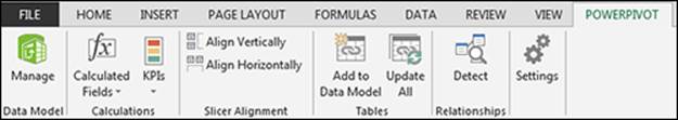
Figure 3-1: After you activate the add-in, you see the Power Pivot tab on the Ribbon.
The Power Pivot Ribbon interface exposes the full set of functionality you don’t get with the standard Data tab. Here are a few examples of functionality available with the Power Pivot interface:
· Browse, edit, filter, and custom sort data import.
· Create custom calculated columns that apply to all rows in your data import.
· Define a default number format to use when the field appears in a PivotTable.
· Configure relationships via a handy graphical diagram view.
· Prevent certain fields from appearing in the PivotTable Field List.
· Configure specific fields to be read as Geography or Image fields.
· Access Key Performance Indicators (KPI).
Linking Excel Tables to Power Pivot
The first step in using Power Pivot is to fill it with data. You can either import data from external data sources or link to Excel tables in your current workbook. See Chapter 4 for more about importing data from external data sources. For now, you can link three Excel tables to Power Pivot.
In this scenario, you have three datasets in three different worksheets (see Figure 3-2):
· The Customers dataset contains basic information like CustomerID, CustomerName, and Address.
· The InvoiceHeader dataset contains data that points specific invoices to specific customers.
· The InvoiceDetails dataset contains the specifics of each invoice.
If you want to analyze revenue by customer and month, you need to join these three tables. In the past, you'd have to go through a series of gyrations involving vlookup or other clever formulas. But with Power Pivot, you can build these relationships in just a few clicks.
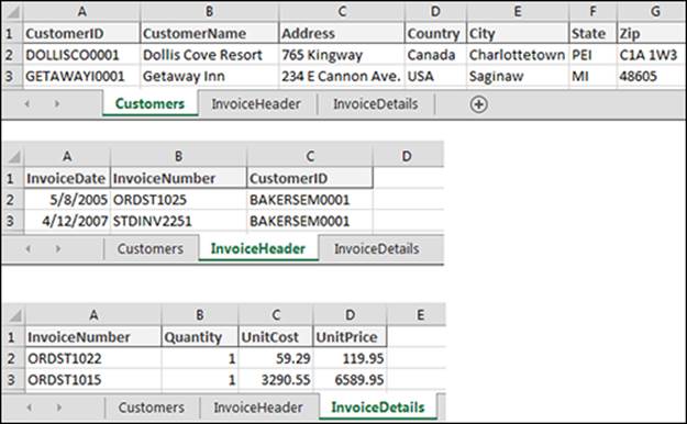
Figure 3-2: Use Power Pivot to analyze the data in the Customers, InvoiceHeader, and InvoiceDetails worksheets.
Preparing your Excel tables
When linking Excel data to Power Pivot, it’s best to first convert your data to explicitly named tables. Although it’s not technically necessary, giving your tables easy-to-remember names helps track and manage your data in the Power Pivot Data Model. If you don't convert your data to tables first, Excel does it for you and gives your tables useless names like Table1 and Table2.
Follow these steps to convert each dataset into an Excel table:
1. On the Customers tab, click anywhere inside the data range.
2. Press Ctrl+T.
3. In the Create Table dialog box, check that the range for the table is correct and that the My Table Has Headers option is selected. Click the OK button.
The Table Tools Design tab appears on the Ribbon.
4. On the Table Tools Design tab, click in the Table Name input and give your table an easy to remember name (see Figure 3-3).
This ensures that you will be able to recognize the table when adding it to the internal Data Model.
5. Repeat Steps 1-4 for the InvoiceHeader and InvoiceDetails datasets.
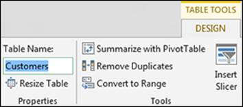
Figure 3-3: Give your newly created Excel table a friendly name.
Adding your Excel tables to the Data Model
After you’ve converted your data to Excel tables, you’re ready to add the tables to the Power Pivot Data Model. Follow these steps to add your new created Excel tables to the Data Model using the Power Pivot tab:
1. Place your cursor anywhere inside your Customers table.
2. On the Power Pivot tab, click the Add to Data Model button.
Power Pivot creates a copy of your table and opens the Power Pivot window (shown in Figure 3-4).
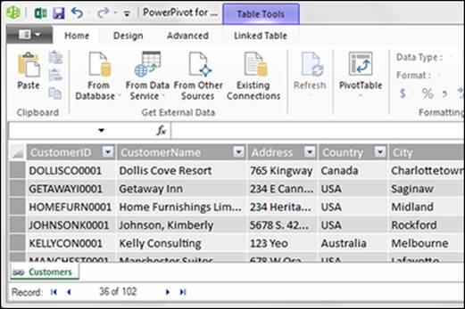
Figure 3-4: The Power Pivot window shows all the data that currently exists in your data model.
3. Repeat Steps 1 and 2 for your other Excel tables: InvoiceHeader and InvoiceDetails.
After you have imported all your Excel tables into the Data Model, your Power Pivot window shows each dataset on its own tab, as shown in Figure 3-5.
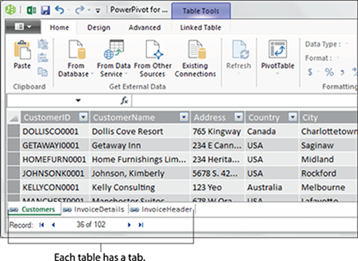
Figure 3-5: Each table you add to the Data Model is placed on its own tab in Power Pivot.
When working with Power Pivot, note the following:
· Although the Power Pivot window looks like Excel, it’s actually a separate program.
· The grid for your table does not have any row or column references.
· You can’t edit the data within the table. This data is simply a snapshot of the actual Excel table you imported.
· You can switch between Excel and the Power Pivot window by clicking each respective program in the taskbar.
![]() The tabs in the Power Pivot window shown in Figure 3-6 have a hyperlink icon next to the tab names. This icon indicates that the data contained in the tab is a linked Excel table. This means that even though the data is a snapshot of the data at the time you added it, the data automatically updates when you edit the source table in Excel.
The tabs in the Power Pivot window shown in Figure 3-6 have a hyperlink icon next to the tab names. This icon indicates that the data contained in the tab is a linked Excel table. This means that even though the data is a snapshot of the data at the time you added it, the data automatically updates when you edit the source table in Excel.
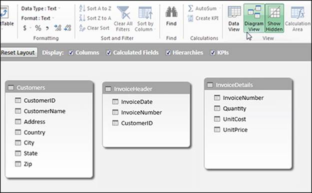
Figure 3-6: The Diagram View allows you to see all the tables in your Data Model.
Creating Relationships Among Your Power Pivot Tables
You can think of a relationship like a vlookup, in which you relate the data in one range to the data in another range using an index or unique identifier. In Power Pivot, you use relationships to do the same thing, but without the hassle of writing a formula.
At this point, Power Pivot knows you have three tables in the Data Model, but it has no idea how these three tables relate to one another. You need to connect these tables by defining relationships among the Customers, InvoiceDetails, and InvoiceHeader tables. You can do so within the Power Pivot window. Follow these steps:
1. Open the Power Pivot window and click the Diagram View button on the Home tab.
![]() If you inadvertently closed the Power Pivot window, you can open it by clicking the Manage button on the Power Pivot tab.
If you inadvertently closed the Power Pivot window, you can open it by clicking the Manage button on the Power Pivot tab.
Power Pivot displays a screen that shows a visual representation of all the tables in the Data Model (see Figure 3-6).
![]() You can move the tables in the Diagram View around by clicking and dragging them.
You can move the tables in the Diagram View around by clicking and dragging them.
The idea is to identify the primary index keys in each table and connect them. In this scenario, the Customers and InvoiceHeader tables can be connected using the CustomerID field. The InvoiceHeader and InvoiceDetails tables can be connected using the InvoiceNumber field.
2. Click and drag a line from the CustomerID field in the Customers table to the CustomerID field in the InvoiceHeader table (as shown in Figure 3-7).
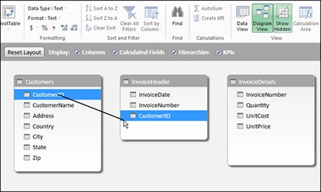
Figure 3-7: To create a relationship, simply click and drag a line between the fields in your tables.
3. Click and drag a line from the InvoiceNumber field in the InvoiceHeader table to the InvoiceNumber field in the InvoiceDetails table.
At this point, your diagram looks similar to Figure 3-8. Notice Power Pivot shows a line between the tables you just connected. In database-speak, these are referred to as joins.
The joins in Power Pivot are always one to many joins. This means that when a table is joined to another, one of the tables has unique records with unique index numbers, while the other can have many records where index numbers are duplicated.
A common example, shown in Figure 3-8, is the relationship between the Customers table and the InvoiceHeader table. In the Customers table, you have a unique list of customers, each with its own identifier. No CustomerID in that table is duplicated. The InvoiceHeader table has many rows for each CustomerID; each customer can have many invoices.
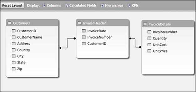
Figure 3-8: When you create relationships, the Power Pivot diagram shows join lines between your tables.
Notice that the join lines have arrows pointing from one table to another. The arrow in these join lines always points to the table that has the non-duplicated unique index.
![]() To close the diagram and get back to seeing the data tables, click the Data View button in the Power Pivot window.
To close the diagram and get back to seeing the data tables, click the Data View button in the Power Pivot window.
If you need to edit or delete a relationship between two tables in your Data Model, you can do so by following these steps:
1. Open the Power Pivot window. On the Design tab, click the Manage Relationships button.
2. In the Manage Relationships dialog box, click the relationship you want to work with and then click Edit or Delete.
Clicking Edit opens the Edit Relationship dialog box shown in Figure 3-9.
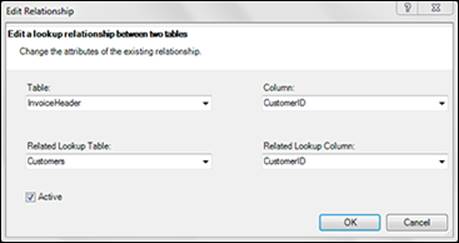
Figure 3-9: Define the relationship by selecting the appropriate table and field names from the drop-down lists.
3. Select the appropriate table and field names from the drop-down lists to redefine the relationship.
4. Click OK when you're done. Click the Close button in the Manage Relationships dialog box to get back to the Power Pivot model.
![]() In Figure 3-9, you see that the lower-left field is called Related Lookup Table. In this drop-down list, you must select the table that contains unique non-duplicated rows. The column you select in the Related Lookup Column must contain unique items.
In Figure 3-9, you see that the lower-left field is called Related Lookup Table. In this drop-down list, you must select the table that contains unique non-duplicated rows. The column you select in the Related Lookup Column must contain unique items.
Creating a PivotTable from Power Pivot Data
After you define the relationships in your Power Pivot Data Model, it’s essentially ready for action. In terms of Power Pivot, “action” means analysis with a PivotTable. Creating a PivotTable from a Power Pivot Data Model is relatively straightforward:
1. Open the Power Pivot window. On the Home tab, click the PivotTable button.
2. Specify whether you want the PivotTable placed on a new worksheet or an existing sheet.
3. Build your needed analysis just as you would any other standard PivotTable, using the Pivot Field List.
Turn to Chapter 2 if you need to configure a PivotTable with the Pivot Field List.
The PivotTable shown in Figure 3-10 contains all the tables in the Power Pivot Data Model. With this configuration, you have a powerful cross-table analytical engine in the form of a familiar PivotTable. From here, you can calculate the average Unit Price by customer.
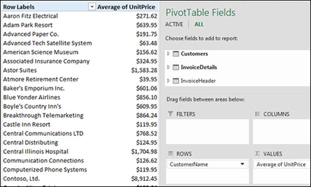
Figure 3-10: You now have a Power Pivot-driven PivotTable that aggregates across multiple tables.
In the days before Power Pivot, this analysis would have been difficult to get to. You needed to build vlookup formulas to get from Customer to Invoice Numbers, then another set of vlookup formulas to get from Invoice Numbers to Invoice Details. And after all that formula building, you still wouldn't have a way to aggregate the data to average Unit Price per customer.
With Power Pivot, you get to your analysis in just a few clicks!
 Limitations of Power Pivot-driven PivotTables
It’s important to note that Power Pivot-driven PivotTables come with some limitations that you don’t encounter with standard PivotTables:
· The Group feature is disabled for Power Pivot-driven PivotTables. You can’t roll dates into months, quarters, years, and so on. You can work around this using your own calculated columns described later in this chapter.
· In a standard PivotTable, you can double-click a cell to drill down to the rows that make up the figure in that cell. In Power Pivot-driven PivotTables, however, you only get the first 1,000 rows.
· Power Pivot-driven PivotTables won’t allow you to create the traditional Calculated Fields and Calculated Items found in standard Excel PivotTables.
· Workbooks that use the Power Pivot Data Model cannot be refreshed or configured if opened in a version of Excel earlier than Excel 2013.
· You cannot use custom lists to automatically sort the data in your Power Pivot-driven PivotTables.
· The Product and Count Numbers summary calculations are not available with Power Pivot-driven PivotTables.
Enhancing Power Pivot Data with Calculated Columns
When analyzing data with Power Pivot, you may need to expand your analysis to include data based on calculations that are not in your original dataset. Power Pivot provides a way to add your own calculations with calculated columns. Calculated columns are columns you create to enhance a Power Pivot table with your own formulas. Calculated columns are entered directly in the Power Pivot window, becoming part of the source data you use to feed your PivotTable. Calculated columns work at the row level; that is, the formulas you create in a calculated column perform their operations based on the data in each individual row. For example, imagine you have a Revenue column and a Cost column in your Power Pivot table. You could create a new column that calculates revenue minus cost. This calculation is simple and valid for each row in the dataset.
Creating a calculated column
Creating a calculated column works very much like building formulas in an Excel table. Follow these steps to create a calculated column:
1. Open the Power Pivot window and click the Invoice Details tab.
![]() If you inadvertently closed the Power Pivot window, you can open it by clicking the Manage button on the Power Pivot Ribbon.
If you inadvertently closed the Power Pivot window, you can open it by clicking the Manage button on the Power Pivot Ribbon.
2. Click in the first blank cell in the Add Column column.
3. Enter the following formula on the formula bar:
=[UnitPrice]*[Quantity]
4. Press Enter to see your formula populate the entire column.
Power Pivot automatically renames the column to CalculatedColumn1.
5. Double-click the column label and rename the column Total Revenue.
Your table now has a calculated column similar to that shown in Figure 3-11.
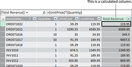
Figure 3-11: Your formula automatically populates all rows in your new calculated column.
6. Create another calculated column called Total Cost.
The formula is =[UnitCost]*[Quantity].
In Figure 3-11, notice how calculated columns are slightly darker than the standard imported columns. This allows you to easily see the calculated columns.
![]() You can rename any column in the Power Pivot window by double-clicking the column name and entering a new name. Alternatively, you can right-click any column and select Rename.
You can rename any column in the Power Pivot window by double-clicking the column name and entering a new name. Alternatively, you can right-click any column and select Rename.
![]() You can build your calculated columns by clicking instead of typing. For example, instead of manually entering =[UnitPrice]*[Quantity], you can enter the equal sign (=), click the UnitPrice column, enter the asterisk (*), and then click the Quantity column. Note that you can also enter your own static data. For example, you can enter a formula to calculate a 10-percent tax rate by entering =[UnitPrice]*1.10.
You can build your calculated columns by clicking instead of typing. For example, instead of manually entering =[UnitPrice]*[Quantity], you can enter the equal sign (=), click the UnitPrice column, enter the asterisk (*), and then click the Quantity column. Note that you can also enter your own static data. For example, you can enter a formula to calculate a 10-percent tax rate by entering =[UnitPrice]*1.10.
After you have your two calculated columns, go back to the PivotTable you created earlier in this chapter (see “Creating a PivotTable from Power Pivot Data”). Take a look at the field list. If you accidentally closed your field list, right-click anywhere in the PivotTable and select Show Field List.
Your newly created calculated columns are now available in the field list, as shown in Figure 3-12. Notice that you didn’t have to take any action to get your calculated columns into the PivotTable. Each calculated column you create is automatically available in any PivotTable connected to the Power Pivot Data Model. You can use these calculated columns just as you would any other field in your PivotTable.
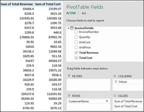
Figure 3-12: Calculated columns automatically show up in the PivotTable Field List.
![]() If you need to edit the formula in a calculated column, find the calculated column in the Power Pivot window, click the column, and then make your changes directly in the formula bar.
If you need to edit the formula in a calculated column, find the calculated column in the Power Pivot window, click the column, and then make your changes directly in the formula bar.
Formatting your calculated columns
You often need to change the formatting of your Power Pivot columns to appropriately match the data within them; for example, to show numbers as currency, remove decimal places, or display dates in a certain way.
You are by no means limited to formatting just calculated columns. You can format any column; just click in the column you want to format and use the tools in the Formatting group on the Home tab of the Ribbon.
![]() Veterans of Excel PivotTables know that changing PivotTable number formats one data field at a time is a pain. One fantastic feature of Power Pivot formatting is that any format you apply to your columns in the Power Pivot window is automatically applied to all PivotTables connected to the Data Model.
Veterans of Excel PivotTables know that changing PivotTable number formats one data field at a time is a pain. One fantastic feature of Power Pivot formatting is that any format you apply to your columns in the Power Pivot window is automatically applied to all PivotTables connected to the Data Model.
Referencing calculated columns in other calculations
Like all calculations in Excel, Power Pivot allows you to reference a calculated column as a variable in another calculated column. Figure 3-13 shows a calculated column called Gross Margin. The formula bar shows the calculation is using the previously created[Total Revenue] and [Total Cost] calculated columns.
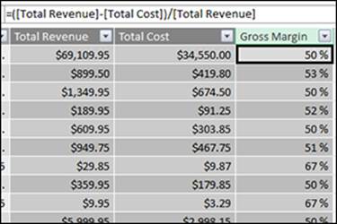
Figure 3-13: The Gross Margin calculation is using the previously created [Total Revenue] and [Total Cost] calculated columns.
Hiding calculated columns from end users
Because calculated columns can reference each other, you can imagine creating columns simply as helper columns for other calculations. You may not want your end users to see these columns in your client tools. In this context, the term “client tools” refers to PivotTables, Power View dashboards, and Power Map.
Similar to hiding columns on an Excel worksheet, Power Pivot allows you to hide any column (it doesn’t have to be a calculated column). To hide columns, select the columns you want hidden, right-click the selection, and then select Hide from Client Tools.
Your selected columns become subdued and grayed out, as shown in Figure 3-14; you can easily identify which columns are hidden.
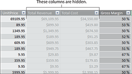
Figure 3-14: The [Total Revenue] and [Total Cost] columns are hidden.
When a column is hidden, it doesn't appear as an available selection in your PivotTable Field List. However, if the column you're hiding is already part of the pivot report, meaning you already dragged it onto the PivotTable, hiding the column doesn't automatically remove it from the report. Hiding it merely affects the ability to see the column in the PivotTable Field List.
![]() To unhide columns, select the hidden columns in the Power Pivot window, right-click the selection, and then select Unhide from Client Tools.
To unhide columns, select the hidden columns in the Power Pivot window, right-click the selection, and then select Unhide from Client Tools.
Utilizing DAX to Create Calculated Columns
DAX (Data Analysis Expression) is the formula language Power Pivot uses to perform calculations within its own construct of tables and columns. The DAX formula language comes with its own set of functions. Some of these functions can be used in calculated columns for row level calculations, while others are designed to be used in calculated fields for aggregate operations.
In this section, we touch on some of the DAX functions that can be leveraged in calculated columns.
Identifying DAX functions that are safe for calculated columns
In the previous section, we showed you how to use the formula bar within the Power Pivot window to enter calculations. Next to that formula bar, you may have noticed the Insert Function button (labeled with an fx). This is similar to the Insert Function button found in Excel. You can browse, search for, and insert the available DAX functions.
Click the fx button and the Insert Function dialog box opens, as shown in Figure 3-15.
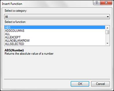
Figure 3-15: The Insert Function dialog box shows you all available DAX functions.
![]() As you look through the list of DAX functions, notice many of them look like the Excel functions you're already familiar with. But make no mistake; these aren’t Excel functions. Where Excel functions work with cells and ranges, these DAX functions are designed to work at the table and column levels.
As you look through the list of DAX functions, notice many of them look like the Excel functions you're already familiar with. But make no mistake; these aren’t Excel functions. Where Excel functions work with cells and ranges, these DAX functions are designed to work at the table and column levels.
To see how these DAX functions work, add a calculated column on the Invoice Details tab. Enter the SUM function SUM([UnitCost]) in the formula bar. The result you get is shown in Figure 3-16.
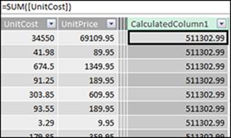
Figure 3-16: The DAX SUM function can only sum the column as a whole.
As you can see, the SUM function sums the entire column. This is because Power Pivot and DAX are designed to work with tables and columns. Power Pivot has no construct for cells and ranges. It doesn’t even have column letters and row numbers on its grid. So where you would normally reference a range (such as in an Excel SUM function), DAX basically takes the entire column.
The bottom line is that you can't use all DAX functions with calculated columns. Because a calculated column evaluates at the row level, only DAX functions that evaluate single data points can be used in a calculated column.
A good rule is that if the function requires an array or a range of cells as an argument, then it’s not viable in a calculated column. So functions such as SUM, MIN, MAX, AVERAGE, and COUNT don’t work in calculated columns. Functions such as YEAR, MONTH, MID, LEFT, RIGHT, IF, and IFERROR that require only single data point arguments are better suited for use in calculated columns.
Building DAX-driven calculated columns
To use a DAX function to enhance calculated columns, click the Invoice Header tab in the Ribbon.
Figure 3-17 contains an InvoiceDate column. Although this column is valuable in the raw table, the individual dates aren’t convenient when analyzing the data with a PivotTable. It would be beneficial to have a column for Month and a column for Year. This way, you could aggregate and analyze data by month and year.
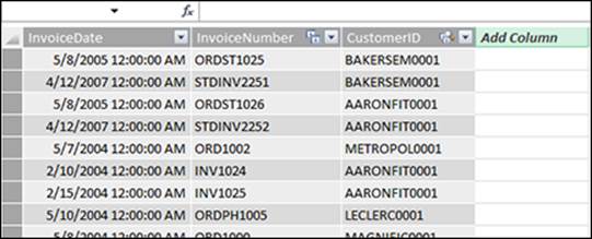
Figure 3-17: Although this table has an InvoiceDate field, adding Year and Month columns would allow for better time-based analysis.
For this endeavor, you use the year(), month(), and format() DAX functions to add time dimensions to your data model. Follow these steps:
1. In the InvoiceHeader table, click in the first blank cell in the Add Column column on the far right.
2. In the formula bar, type =YEAR([InvoiceDate]) and press Enter.
Power Pivot automatically names the column CalculatedColumn1.
3. Double-click the CalculatedColumn1 column label and rename the column Year.
4. Repeat Steps 1-3 to add two additional columns:
· Month: Enter =MONTH([InvoiceDate]) in the formula bar and rename the column Month.
· Month Name: Enter =FORMAT([InvoiceDate],”mmm”) in the formula bar and rename the column Month Name.
You now have three new calculated columns similar to those shown in Figure 3-18.
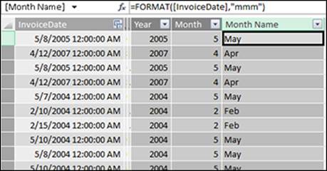
Figure 3-18: Using DAX functions to supplement a table with Year, Month, and Month Name columns.
As mentioned previously, creating calculated columns automatically makes them available through your PivotTable Field Lists (see Figure 3-19).
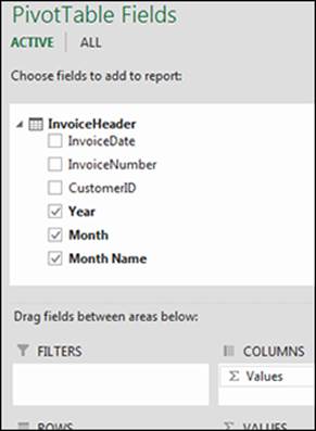
Figure 3-19: DAX calculations are immediately available in any connected PivotTable.
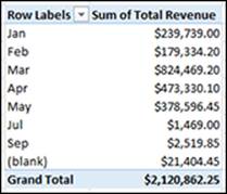
Month sorting in Power Pivot-driven PivotTables
One of the more annoying things about Power Pivot is that it doesn’t inherently know how to sort months. Unlike standard Excel, Power Pivot doesn’t use the built-in custom lists that define the order of month names. So when you create a calculated column like [Month Name] and place it into your PivotTable, Power Pivot puts those months in alphabetical order.
The fix for this is fairly easy. Open the Power Pivot window and click the Sort by Column button.
In the Sort by Column dialog box, select the column you want sorted, and then select the column you want to sort by.
Click OK, and you might think you did something wrong because nothing happens. This is because the sort order you defined is not for the Power Pivot window. The sort order is applied to your PivotTable. Switch to Excel to see the result in the PivotTable.
Understanding Calculated Fields
You can enhance the functionality of your Power Pivot reports with another kind of calculation called a calculated field. Calculated fields are used to perform more complex calculations that work on an aggregation of data. These calculations are not applied to the Power Pivot window like calculated columns. Instead, they're applied directly to your PivotTable, creating a sort of virtual column that can’t be seen in the Power Pivot window. You use calculated fields when you need to calculate based on an aggregated grouping of rows.
Imagine you wanted to show the dollar variance between the years 2007 and 2006 for each of your customers. Think about what technically has to be done to achieve this calculation. You’d have to figure out the sum of revenue for 2007, then you’d have to get the sum of revenue for 2006, then you’d have to subtract the sum of 2007 from the sum of 2006. This is a calculation that simply can’t be done using calculated columns. Using calculated fields is the only way to get the dollar variance between 2007 and 2006.
Follow these steps to create a calculated field:
1. Start with a PivotTable created from a Power Pivot model.
2. Click the Power Pivot tab on the Ribbon and choose Calculated Fields → New Calculated Field.
The Calculated Field dialog box opens, as shown in Figure 3-20.
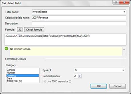
Figure 3-20: Creating a new calculated field.
3. Set the following inputs:
· Table Name: Choose the table that will contain the calculated field when looking at the PivotTable Fields list.
· Calculated Field Name: Give your calculated field a descriptive name.
· Formula: Enter the DAX formula that will calculate the results of your new field.
· Formatting Options: Specify the formatting for the calculated field results.
In this example, we use the following DAX formula:
=CALCULATE(SUM(InvoiceDetails[Total Revenue]),
InvoiceHeader[Year]=2007)
This formula uses the Calculate function to sum the Total Revenue column from the InvoiceDetails table, where the Year column in the InvoiceHeader is equal to 2007. This is just one of a limitless number of formulas you can use to define a calculated field.
4. Click the Check Formula button to ensure there are no syntax errors.
If your formula is well formed, you see the message No errors in formula. If there are errors, you see a full description of the errors.
5. Click OK to confirm your changes and close the Calculated Field dialog box.
You immediately see your newly created calculated field in the PivotTable.
6. Repeat Steps 2-5 for any other calculated field you need to create.
In this example, we created two additional calculated fields:
=CALCULATE(SUM(InvoiceDetails[Total Revenue]),InvoiceHeader[Year]=2006)
=[2007 Revenue]-[2006 Revenue]
Figure 3-21 shows the newly created calculated fields. The calculated fields are applied to each customer, showing the variance between their 2007 and 2006 revenues. Note that once you create calculated fields, they're available for selection in the PivotTable Fields list.
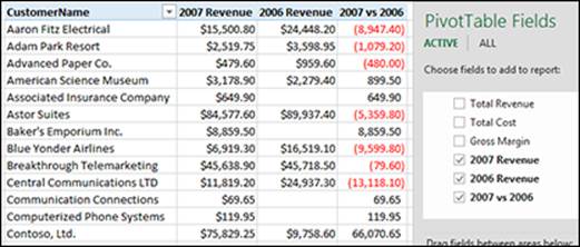
Figure 3-21: Calculated fields can be seen in the PivotTable Fields list.
![]() There are over 140 different DAX functions. You can click the fx button in the Calculated Field dialog box to see all the available DAX functions that can be used to implement a new calculated field. A full overview of DAX is out of the scope of this book. If after reading this section, you have a desire to learn more about DAX, consider picking up Microsoft Excel 2013: Building Data Models with PowerPivot, by Alberto Ferrari and Marco Russo (Microsoft Press).
There are over 140 different DAX functions. You can click the fx button in the Calculated Field dialog box to see all the available DAX functions that can be used to implement a new calculated field. A full overview of DAX is out of the scope of this book. If after reading this section, you have a desire to learn more about DAX, consider picking up Microsoft Excel 2013: Building Data Models with PowerPivot, by Alberto Ferrari and Marco Russo (Microsoft Press).
You may find that you need to either edit or delete a calculated field. You can do so by following these steps:
1. Click anywhere inside your PivotTable, then click the Power Pivot tab on the Ribbon and choose Calculated Fields → Manage Calculated Fields.
The Manage Calculated Field dialog box opens, as shown in Figure 3-22.
2. Select the target calculated field and click either the Edit or Delete button.
Clicking the Edit button opens the Calculated Field dialog box, where you can make changes to the calculation setting. Clicking the Delete button opens a message box asking you to confirm that you want to remove the calculated field.
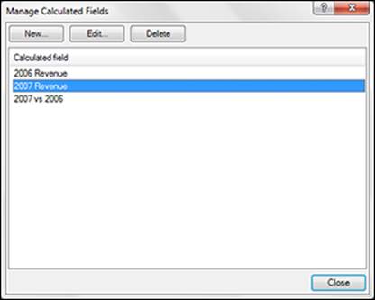
Figure 3-22: The Manage Calculated Fields dialog box lets you edit or delete your calculated fields.
All materials on the site are licensed Creative Commons Attribution-Sharealike 3.0 Unported CC BY-SA 3.0 & GNU Free Documentation License (GFDL)
If you are the copyright holder of any material contained on our site and intend to remove it, please contact our site administrator for approval.
© 2016-2026 All site design rights belong to S.Y.A.