Microsoft Office 2016: The Complete Guide (2015)

HOW TO CREATE A PIVOTTABLE IN EXCEL 2016 TO EVALUATE WORKSHEET INFORMATION

A PivotTable is essential for large quantities of data. When using Excel; it recommends and automatically creates a PivotTable so that you can easily summarize all your data. Being able to analyze all the data in your worksheet can help you make better business decisions.

How to create a Recommended PivotTable?

If you have limited experience with PivotTables, or are not sure how to get started, a Recommended PivotTable is a good choice. When you use this feature, Excel determines a meaningful layout by matching the data with the most suitable areas in the PivotTable. This helps give you a starting point for additional experimentation. After a basic PivotTable is created, you can explore different orientations and rearrange fields to achieve your specific results.

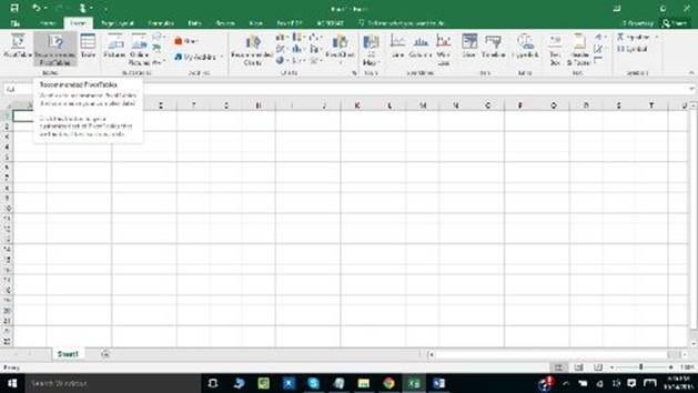
Bring up the workbook where the Pivot Table will be created.

Select the cell which has the information that will be used in the PivotTable.

Go to the Insert tab and select the option Recommended PivotTables.

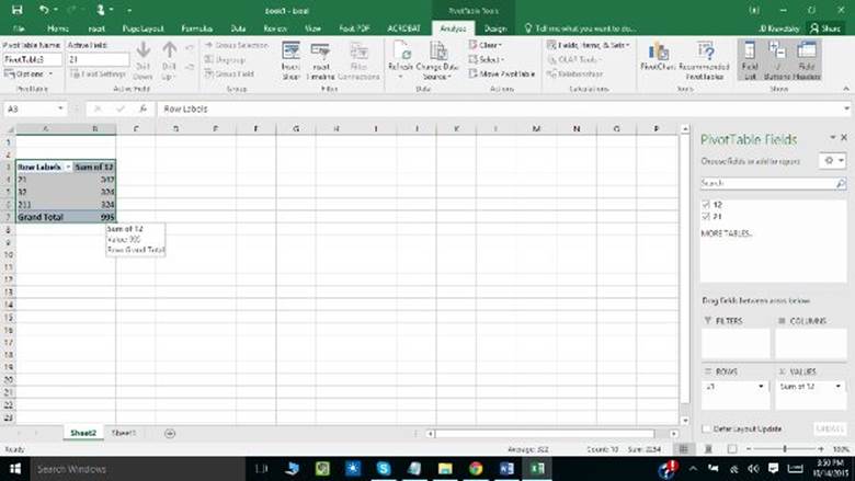
Excel generates a PivotTable on a different sheet and shows the PivotTable Fields List.

To insert a nee field, go to the FIELD NAME area and mark the check box for the field. Nonnumeric fields are automatically sent to the Row area, while the Column area contains the date and time hierarchies. Data that is numeric goes to the Values area.

To remove a field, go to the FIELD NAME option and uncheck the check box for that particular field.

To transfer a field, Drag the field from one area of the PivotTable Fields List to another, for example, from Columns to Rows.

To Refresh the PivotTable: On the PivotTable Analyze tab, click Refresh.

How to create a PivotTable manually

A Pivot Table can be created manually, given that you are familiar with and know the particular arrangement for your data.

Bring up the workbook where the Pivot Table will be created.

Select the cell which has the information that will be used in the PivotTable.

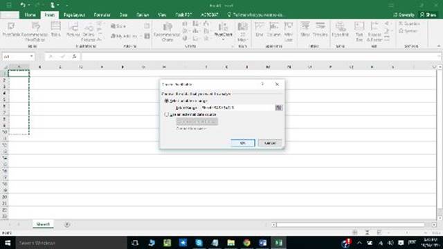
Go to the Insert tab and select the option PivotTable.

A dashed line should surround the data in your worksheet. If that is absent, click and drag the highlighted data. This will automatically fill the Table/Range box with your designated cell range.

The option Choose where you want the PivotTable report to be placed, will appear, select New worksheet if you wish to place the PivotTable on a new worksheet tab. Or, select Existing worksheet, and select where it should be placed.

TIP By checking the Add this data to the Data Model box, you can analyze several tables in a PivotTable.

Select OK.