Office 2016 For Seniors For Dummies (2016)

Part III

Excel

For an explanation of Excel's IF function, visit www.dummies.com/extras/office2016forseniors.

Chapter 8

Doing the Math: Formulas and Functions

Get ready to . . .

Learn How Formulas Are Structured

Write Formulas That Reference Cells

Move and Copy Cell Content

Reference a Cell on Another Sheet

Understand Functions

Take a Tour of Some Basic Functions

Explore Financial Functions

The main reason why people choose Excel is that it “excels” at storing and calculating numeric data. With Excel, you can create a grid of numbers, and then insert formulas that perform math calculations on them. That capability makes it possible to build complex worksheets that calculate loan rates and payments, keep track of your bank accounts, and much more.

In this chapter, I show you how to build formulas and functions in Excel, and how to put them to work to do several types of calculation-based jobs.

Learn How Formulas Are Structured

A formula is a math calculation, like 2 + 2 or 3(4 + 1). In Excel, formulas are different from regular text in two ways:

· They begin with an equal sign, like this: =2+2

· They don’t contain text (except for function names, covered later, and cell references). They contain only symbols that are allowed in math formulas, such as parentheses, commas, and decimal points.

Just like in basic math, formulas are calculated by using an order of precedence. Table 8-1 lists the order.

Table 8-1 Order of Precedence in a Formula

Write Formulas That Reference Cells

One of Excel’s best features is its ability to reference cells in formulas. When a cell is referenced in a formula, whatever value it contains is used in the formula. When the value changes, the result of the formula changes, too.

For example, suppose you enter 7 in cell A1 and 8 in cell A2. Then in cell A3, you put the following formula:

=A1+A2

The result of that formula appears in cell A3 as 15. See Figure 8-1. You could have just as easily entered =7+8 in cell A3 and gotten the same result. However, because you reference the cells — rather than the fixed values — you can modify the result by changing what either A1 or A2 contains. For example, if you change the value in A1 to 4, the result in A3 changes to 12.

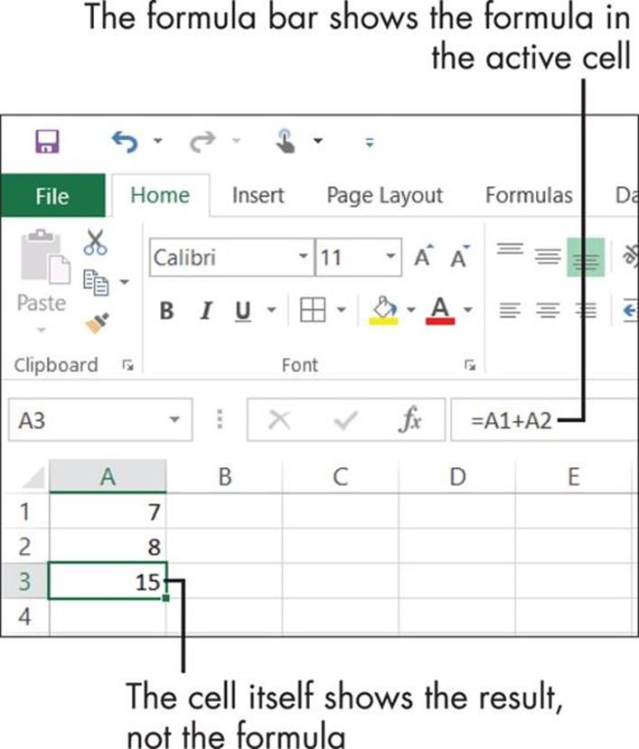
Figure 8-1

You can use a formula to repeat a value between one cell and another. For example, the formula =A1 repeats whatever value is in cell A1 wherever you put it.

You can combine cell references with fixed numbers in cells, too. Here are some examples:

=A1+2
=(A1*A2)/4
=(A1+A2+B1+B2)/4

Move and Copy Cell Content

When you’re creating a spreadsheet, it’s common to not get everything in exactly the right cells to begin with. Fortunately, moving content between cells is easy.

Here are the two methods you can use to move content. Remember to first select the cell(s).

· Clipboard: Choose Home ⇒ Clipboard ⇒ Cut or press Ctrl+X. Then click the destination cell and choose Home ⇒ Clipboard ⇒ Paste or press Ctrl+V. If you want to copy rather than move, choose Copy (Ctrl+C) rather than Cut.

If you’re moving or copying a multi-cell range with the Clipboard method, you can either select the same size and shape of block for the destination. Or you can select a single cell, and the paste will occur with the selected cell in the upper-left corner.

· Mouse: Point at the dark outline around the selected range, and then drag to the new location. If you want to copy rather than move, hold down the Ctrl key while you drag. See Figure 8-2.

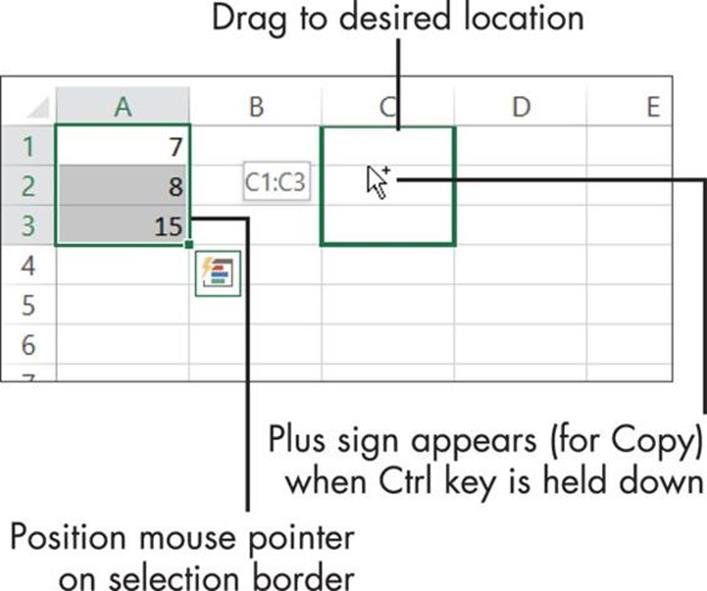
Figure 8-2

When you move or copy a formula, Excel automatically changes the cell references to work with the new location. For example, suppose you copy the formula in cell A3 (from Figure 8-1) into cell C3. The original formula was =A1+A2. When it arrives at C3, it changes to =C1+C2. This happens by design, as a convenience to you, because often when you copy formulas, you want them to work relative to their new locations. This is called a relative reference.

Sometimes, you might not want the cell references in a formula to change when you move or copy it. In other words, you want it to be an absolute reference to that cell. To make a reference absolute, you add dollar signs before the column letter and before the row number. So, for example, an absolute reference to C1 would be =$C$1.

You can mix relative and absolute references in the same formula. For example, in Figure 8-3, if I copy the formula from D4 to D5, the version in D5 will appear like this:

=C5+(C5*$B$1)

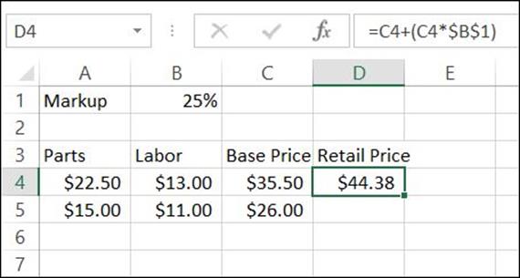
Figure 8-3

The C4 reference changed to C5 because it didn’t have any dollar signs around it, but the B1 reference stayed the same because it did have the dollar signs.

Reference a Cell on Another Sheet

In a multi-sheet workbook, you might want to refer to a cell on a different sheet. To do this, you put the sheet name and an exclamation point in front of the cell reference. For example, to refer to cell A1 on Sheet2, you would write it like this:

=Sheet2!A1

The default sheet names (Sheet1, Sheet2, and so on) have no spaces in the names. If you rename a sheet with a name that includes spaces, you have to put the sheet name in single quotation marks, like this:

=’Home Budget’!A1

Understand Functions

Sometimes, it’s awkward or lengthy to write a formula to perform a calculation. For example, suppose you want to sum the values in cells A1 through A10. To express it as a formula, you would have to write out each cell reference individually, like this:

=A1+A2+A3+A4+A5+A6+A7+A8+A9+A10

In Excel, a function refers to a certain math calculation. Functions can greatly shortcut the amount of typing you have to do to create a particular result. For example, instead of the using the preceding formula, you could sum, using the SUM function like this:

=SUM(A1:A10)

With a function, you can represent a range with the upper-left corner’s cell reference, a colon, and the lower-right corner’s cell reference. In the case of A1:A10, there is only one column, so the upper left is A1 and the lower right is A10.

Each function has one or more arguments. An argument is a placeholder for a number, text string, or cell reference. For example, the SUM function requires at least one argument: a range of cells. So in the preceding example, A1:A10 is the argument. The arguments for a function are enclosed in a set of parentheses.

Each function has its own rules as to how many required and optional arguments it has, and what they represent. You don’t have to memorize the sequence of arguments (the syntax) for each function; Excel asks you for them. It can even suggest a function to use for a certain situation if you aren’t sure what you need.

To find a function and get help with its syntax, follow these steps:

1. Click in the cell where you want to insert the function.

2. Choose Formulas ⇒ Function Library ⇒ Insert Function. The Insert Function dialog box opens.

If you don’t know what function you want, type a few keywords (in the Search for a Function field) that represent what you want to do. For example, if you want to find the minimum value in a range of cells, you might type Find the minimum value. Then click Go to see a list of functions that might be what you want. See Figure 8-4. Click each function on the list and read the description of it that appears.

3. When you find the function you want, click OK.

4. In the Function Arguments dialog box that opens, fill in the arguments in the field provided. The arguments will be different depending on the function you choose. Figure 8-5 shows the arguments for the MIN function, for example.

Here are some ways to fill in the arguments:

· Type a number or a cell reference (or range) directly into the box.

Even though the argument is named Number1 in Figure 8-5, you can still enter a range for it. The Number2 argument is optional; you can tell because its name is not bold. This particular function can have an unlimited number of optional arguments; more boxes appear automatically as needed.

· Click the Selector button to the right of the text box. This collapses the dialog box temporarily. Select the cell or range in the worksheet, and then press Enter to return to the dialog box.

5. Click OK.

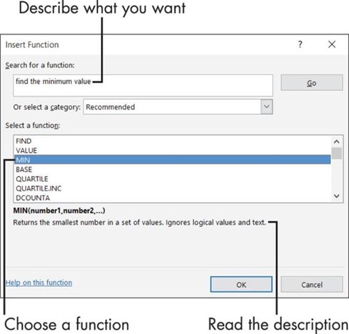
Figure 8-4

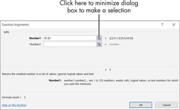
Figure 8-5

After you get comfortable with a particular function, you might prefer to type it directly into the cell rather than going through the Insert Function dialog box. As you type, Excel helps you by providing prompts for the arguments in a ScreenTip. See Figure 8-6.

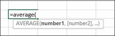
Figure 8-6

Take a Tour of Some Basic Functions

Excel has hundreds of functions, but most of them are very specialized. The basic set that the average user works with is much more manageable.

Start with the simplest functions of them all: those with no arguments. Two prime examples are

· NOW: Reports the current date and time.

· TODAY: Reports the current date.

Even though neither uses any arguments, you still have to include the parentheses, so they look like this:

=NOW( )
=TODAY( )

Another basic kind of function performs a single, simple math operation and has a single argument that specifies what cell or range it operates on. Table 8-2 summarizes some important functions that work this way.

Table 8-2 Simple One-Argument Functions

Table 8-3 shows some functions that change how numbers are presented.

Table 8-3 Functions That Change Numbers

Here are some things to note about the items in the preceding table:

· Absolute value: This is the positive version of a number. For example, the absolute value of -15 is 15. If the number is already positive, it stays positive.

· Multiple arguments: See the entry for ROUND. There are two arguments: the cell address or number to operate on, and the number of decimal places. A value of 0 for the decimal places results in rounding to the nearest integer.

When a function has more than one argument, the arguments are separated by commas. You can see this in the ROUND example: ROUND(B1,0).

Two other functions, ROUNDUP and ROUNDDOWN, work just like ROUND except they specify which way the rounding will always occur.

Explore Financial Functions

Financial functions are some of the most useful tools for home and small business worksheets because they’re all about the money: borrowing it, lending it, and monitoring it. Here’s the basic set:

· PV: Calculates the present value or principal amount. In a loan, it’s the amount you’re borrowing; in a savings account, it’s the initial deposit.

· FV: The future value. This is the principal plus the interest paid or received.

· PMT: The payment to be made per period. For example, for a mortgage, it’s the monthly payment; in a savings account, it’s the amount you save each period. A period can be any time period, but it’s usually a month.

· RATE: The interest rate to be charged per period (for a loan), or the percentage of amortization or depreciation per period.

· NPER: The number of periods. For a loan, it’s the total number of payments to be made, or the points in time when interest is earned if you’re tracking savings or amortization.

These financial functions are related. Each is an argument in the others; if you’re missing one piece of information, you can use all the pieces you do know to find the missing one. For example, if you know the loan amount, the rate, and the number of years, you can determine the payment.

Take a look at the PMT function as an example. The syntax for the PMT function is as follows, with the optional parts in italics:

PMT(RATE, NPER, PV, FV, Type)

The Type argument specifies when the payment is made: 1 for the beginning of the period or 0 at the end of the period. It’s not required. (I don’t use it in the examples here.)

So, for example, say the rate is 0.833% per month (that’s 10% per year), for 60 months, and the amount borrowed is $25,000. The Excel formula looks like this:

=PMT(.00833,60,25000)

Enter that into a worksheet cell, and you’ll find that the monthly payment will be $531.13. You could also enter those values into cells, and then refer to the cells in the function arguments, like this (assuming you entered them into B1, B2, and B3):

=PMT(B1,B2,B3)

Here is the syntax for each of the above-listed functions. As you can see, they’re all intertwined with one another:

FV(RATE, NPER, PMT, PV, Type)
PMT(RATE, NPER, PV, FV, Type)
RATE(NPER, PMT, PV, FV, Type)
NPER(RATE, PMT, PV, FV, Type)

Here are some common ways to use Excel functions in everyday life:

If I borrow $10,000 for 3 years at 7% yearly interest, what will my monthly payments be?

Use the PMT function. Divide the interest rate by 12 because the rate is yearly, but the payment is monthly. Here is the syntax:

=PMT(0.07/12,36,10000)

If I borrow $10,000 at 7% interest and I can afford to make payments of $300 per month, how many months will it take to pay off the loan?

Use the NPER function. Again, divide the interest rate by 12 to convert from yearly to monthly. Here’s the syntax:

=NPER(0.07/12,300,10000)

If I deposit $10,000 into a bank account that pays 2% interest per year, compounded weekly, how much money will I have after 5 years?

You want the future value of the account, or FV. The period is weekly, so the interest rate should be divided by 52, and the length of the loan is 260 periods (52 weeks multiplied by 5 years). The PMT amount is 0 because no additional deposits will be made after the initial deposit. The initial deposit is expressed as a negative number because the calculation is from the perspective of the interest earner, not the interest payer. Here is the syntax:

=FV(0.02/52,260,0,-10000)

As a final example, let’s return to that mortgage spreadsheet I started in Chapter 7 and fill in some numbers, as in Figure 8-7. I’ve annotated each field to explain what I put into each one.

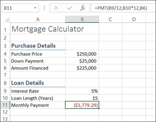
Figure 8-7

It’s all pretty self-explanatory, except the PMT function in cell B11:

=PMT(B9/12,B10*12,B6)

The PMT function requires these three arguments:

· Rate (RATE): For the rate, I use B9/12 because I want to calculate a monthly payment, and the amount in B9 is per year. The interest rate per month is of the interest rate per year.

· Number of periods (NPER): The number in B10 is years, and there are 12 periods (months) in each year — so I multiply B10 by 12.

· Present value (PV): For the present value, I simply refer to B6, which contains the amount to be financed.

This example is especially useful because it shows how a function can be modified to fit a situation. In this case, I had to convert from years (which is how most people think about loans) to months (which is how Excel calculates loans).

One more thing: did you notice that the payment is negative in cell B11? To make it a positive number, I could have enclosed the function in an absolute value function: ABS. Then it would have looked like this:

=ABS(PMT(B9/12,B10*12,B6))

When one function is nested inside another, there is only one equal sign, at the very beginning.