Microsoft Office 2016 At Work For Dummies (2016)

Chapter 9

Formatting and Printing Excel Worksheets

In This Chapter

Applying and customizing themes

Applying a worksheet background

Resizing rows and columns

Applying cell borders and shading

Formatting cells using styles

Using conditional formatting

Setting up headers and footers

Printing a worksheet

Face it: Plain worksheets aren’t that much to look at. A worksheet packed full of rows and columns of numbers is enough to make anyone’s eyes glaze over. However, formatting can dramatically improve a worksheet’s readability, which in turn enables the reader to understand its meaning much more easily.

You can apply formatting at the whole-worksheet level or at the individual-cell level. This lesson focuses on formatting entire worksheets — or at least big chunks of them. You learn how to adjust rows and columns, apply worksheet backgrounds, create headers and footers, and format ranges as tables, complete with preset table formatting. You also learn how to print your work in Excel.

Apply and customize themes

Themes are formatting presets that you can apply to entire worksheets to change their formatting without having to select each formatting aspect manually. A theme includes font, color, and effect choices. You learned about themes in Word in Chapter 2, and themes work basically the same way in Excel, too (and also in PowerPoint, as you’ll see in Chapter 15). The theme choices are the same across those three applications, so you can standardize your formatting across all the documents you create, regardless of application used.

A theme doesn’t override manually applied formatting. It simply redefines the default values for fonts, colors, and effects. In order for a theme’s fonts to apply to a certain cell, you must not have changed its font manually, or you must have changed it to one of the fonts in the Theme Fonts section of the Font drop-down list. Similarly, in order for colors to take effect, you must have recolored objects only with the theme colors placeholders, not with fixed colors. See Chapter 2 for more information. If a cell or object doesn’t appear to be working with the applied theme, select it and choose Home  ⇒  Clear  ⇒  Clear Formats.

Apply a theme

To apply a theme, do the following:

On the Page Layout tab, click Themes. The Themes menu appears.

Click the desired theme.

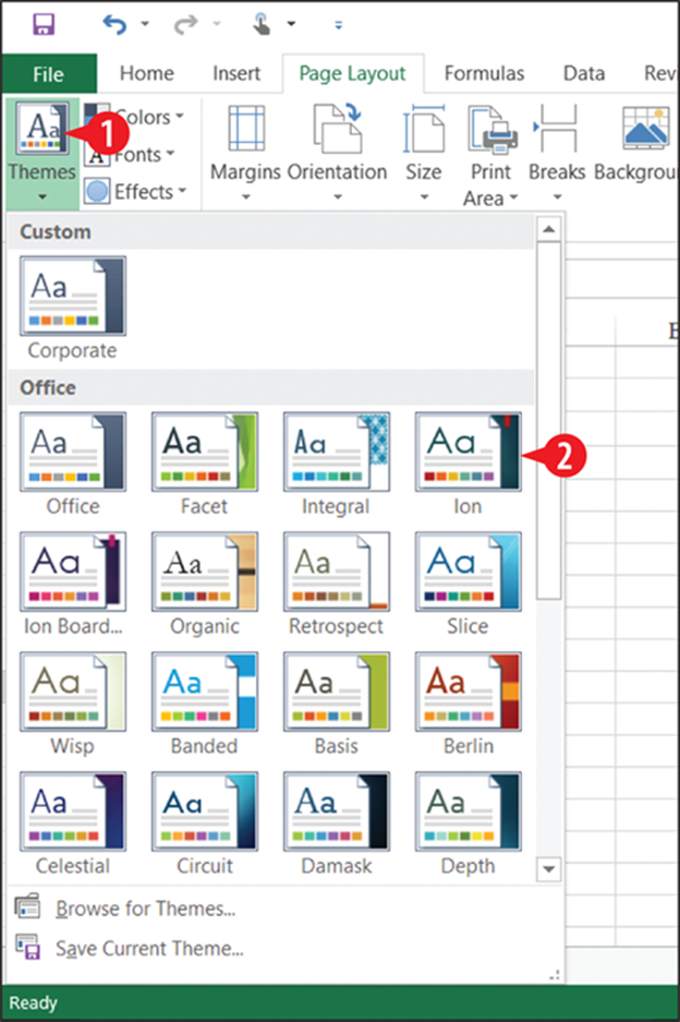
Figure 9-1: Choose a different theme to change the formatting.

Each aspect of a theme can also be individually changed, using the Colors, Fonts, and Effects buttons on the Page Layout tab. Each one opens a menu from which you can make your selection. These color, font, and effect schemes do not correspond one-to-one with the themes on the Themes button’s list; there are more color, font, and effect schemes than there are themes. You can change these as follows:

Click Colors and choose a different set of colors.

Click Fonts and choose a different set of fonts.

Click Effects and choose a different effect type.

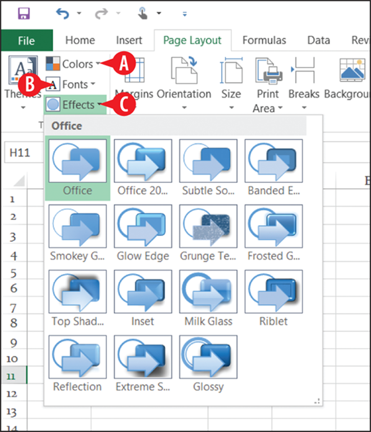
Figure 9-2: Change one aspect of a theme individually from the Design tab.

Effects apply only to certain graphic objects, such as drawn lines and shapes and SmartArt. Therefore, you should not expect to see an immediate, dramatic difference in your worksheet when you apply a different Effect setting unless your worksheet contains graphic objects and those graphic objects have not been manually formatted with specific effects.

Create a custom theme

You can create your own custom themes and then save them and share them with other people. This is handy when your company has specific fonts and colors that you are expected to use in your work-related projects; you can create a theme that uses the right formatting, and then everyone in your company can use that same theme, ensuring consistency.

To create a custom theme, follow these steps:

1. Make your selection of Color, Fonts, and Effects, as in Figure 9-2. If none of the font and color themes are suitable, you can create your own custom schemes, as I explain in the next two sections.

On the Page Layout tab, click Themes, and then click Save Current Theme.

3. In the Save Current Theme dialog box, type a name in the Filename box for the new theme. Leave the save location as-is.

Click Save.

From now on, your custom theme appears on the Themes button’s menu, in the Custom section, as shown at in Figure 9-5.

If you want to share the theme with others, repeat steps 1-4 but this time navigate to a shared location before clicking Save. Excel will save a copy of it there.

If you want to use someone else’s custom theme, click the Themes button and click Browse for Themes. Navigate to the file’s location and click Open. (See in Figure 9-5.)

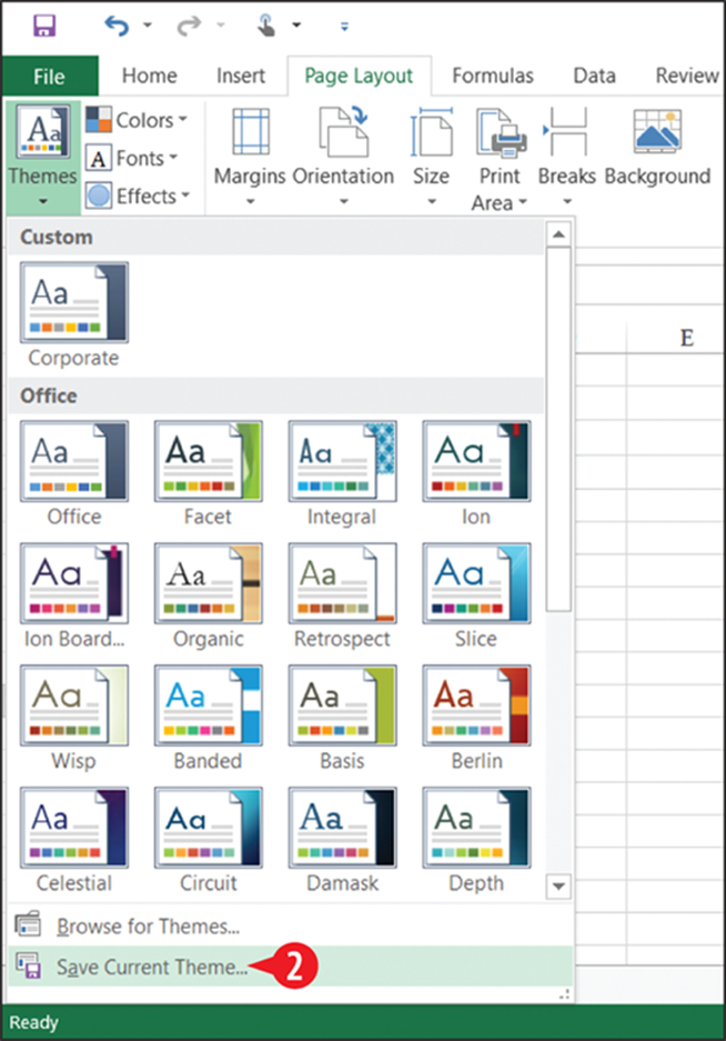
Figure 9-3: Select the Save Current Theme command from the menu.

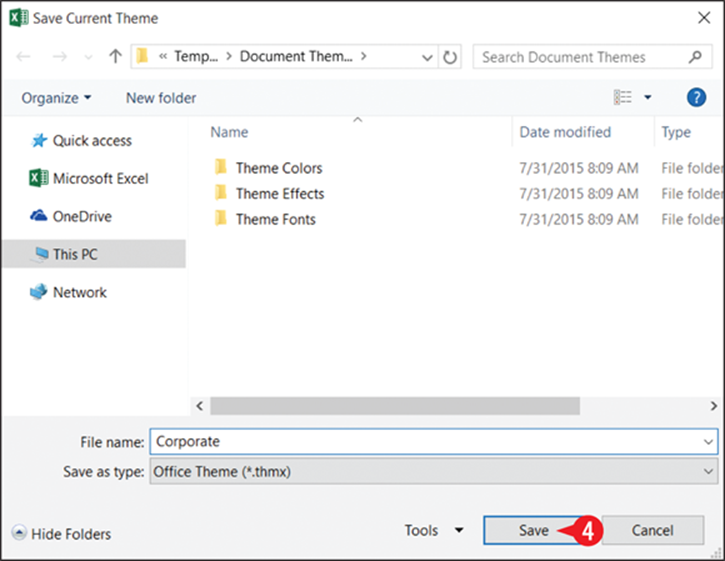
Figure 9-4: Save a custom theme to Excel’s default location for themes.

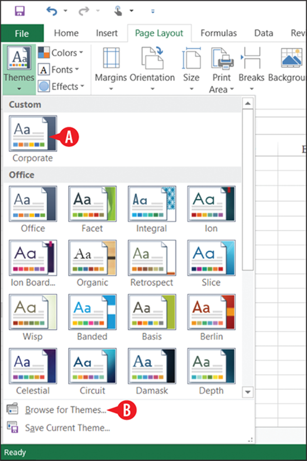
Figure 9-5: Custom themes appear at the top of the menu.

Create a custom color scheme

As you learned in Chapter 2, each color scheme in Office applications consists of values for 12 color placeholders. Each of the preset color combinations is represented on the Colors button’s menu.

To create your own color combination, follow these steps:

On the Page Layout tab, click Colors.

Click Customize Colors.

For each of the 12 placeholders, click its arrow and then choose the desired color.

In most cases you will want to choose one of the colors in the Standard Colors area, or click More Colors for a wider selection. (See in Figure 9-7.)

If you choose a color that is in the Theme Colors section, the color choice will not hold when you apply a different color theme or choose different colors for the other placeholders. (See in Figure 9-7.)

In the Name box, type a name for the custom color scheme.

Click Save.

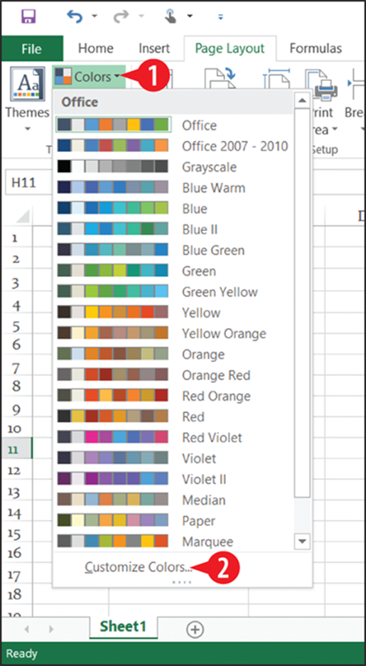
Figure 9-6: Choose Customize Colors from the menu.

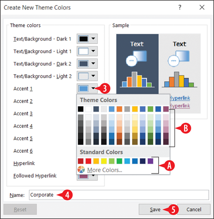
Figure 9-7: Select the desired color for each of the placeholders.

Create a custom font scheme

A font scheme consists of font choices for two types of text: Headings and Body. You can define these placeholders with the same font or two different fonts.

To create a custom font scheme:

On the Page Layout tab, click Fonts.

Click Customize Fonts.

Open the drop-down list for the Heading font and choose a font.

Open the drop-down list for the Body font and choose a font.

Type a name for the scheme in the Name box.

Click OK.

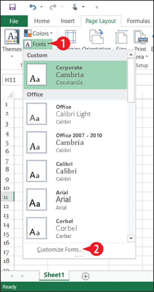
Figure 9-8: Choose the Customize Fonts command.

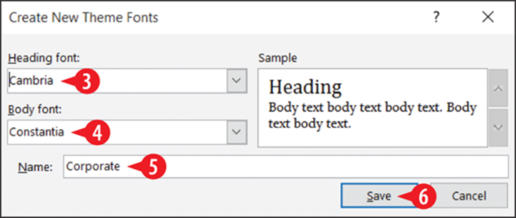
Figure 9-9: Define the fonts for the custom scheme.

Should you wish to share your custom font or color schemes with others, you can find them in C:\Users\username\AppData\Roaming\Microsoft\Templates\Document Themes, in the Theme Colors or Theme Fonts folders, respectively. (Replace username in that path with your Windows username. Browse the C:\Users folder if you don’t know the exact name.)

Apply a worksheet background

A worksheet background is a background picture that appears only onscreen; it doesn’t print. Some people use a background to dress up the appearance of a sheet, but be careful not to impede readability when using one.

As Excel defines it, a “background” is a picture. If you want a solid-color background, apply the same shading to the entire worksheet. You’ll learn about cell shading later in this chapter, in “Apply cell borders and shading.”

A background picture repeats (tiles) itself as needed to fill the entire worksheet. You can’t modify that behavior to stretch the picture or make it repeat only once. (Are you getting the idea yet that a background is a pretty simple, limited feature? It is.)

To apply a picture background:

On the Page Layout tab, click Background. The Insert Pictures dialog box opens.

2. Do one of the following:

Click Browse next to From a File to browse your computer for the picture to use.

Click in the Search Bing box, type a keyword to use for an Internet image search, and press Enter to initiate the search.

Click Browse next to OneDrive to browse your OneDrive storage for the picture to use.

Select the desired picture. (If you chose option or in step 2, you might need to browse for it.)

Click Insert.

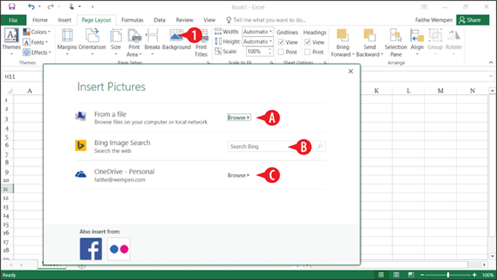
Figure 9-10: Select a source from which to locate an image.

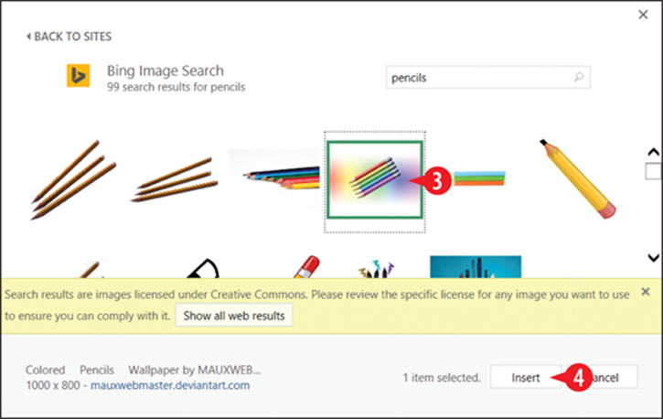
Figure 9-11: Select the desired image.

To remove a background image, choose Page Layout  ⇒  Remove Background.

If you want a background picture that prints, add a picture to the header or footer. You’ll learn about headers and footers later in this chapter, in “Set up headers and footers.” After entering the header/footer for editing, use the Header & Footer Tools Design  ⇒  Picture command to insert a picture in the header or footer. A code appears in the header or footer, but the image itself appears behind the worksheet.

Apply cell borders and shading

Borders and shading are two ways of dressing up a cell’s plain appearance. Here are some tips for using them:

A border is a line around one or more sides of a cell. Not all sides of a cell necessarily have a border. For example, in Figure 9-12 only the top and bottom of this cell have a border. Borders print with the worksheet.

Don’t confuse borders with gridlines, which are the lines onscreen that mark where one cell ends and the next one begins.

To turn off the display of gridlines onscreen, clear the View check box in the Gridlines section of the Page Layout tab.

Gridlines do not print by default. To force gridlines to print, mark the Print check box in the Gridlines section.

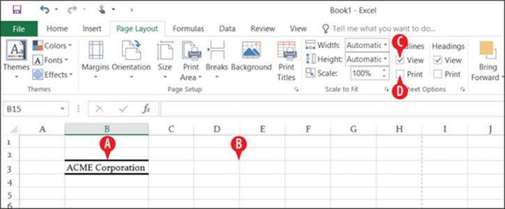
Figure 9-12: Borders versus gridlines

To apply a border:

Select the cell or range that should receive the border.

Click the arrow on the Borders button on the Home tab, opening a menu.

If you don’t want the default colored line (black), point to Line Color and then select the desired color (if not black, the default).

If you don’t want the default line style (solid thin line), reopen the Borders button’s menu, point to Line Style, and click the desired line style.

5. Reopen the Borders button menu if needed. Then click the type of border in the Borders section of the menu:

The Outside border, when applied to a multi-cell range, creates a single border around the range.

All Borders applies the border to every side of every cell in the range.

Some of the possible styles include solid (thin), solid (thick), dotted, and dashed (in various patterns).

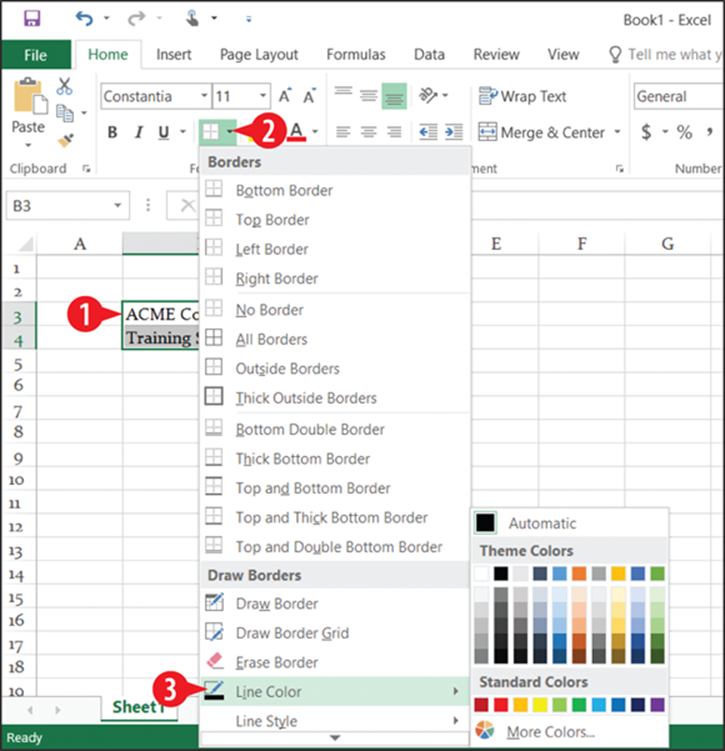
Figure 9-13: Select a line color.

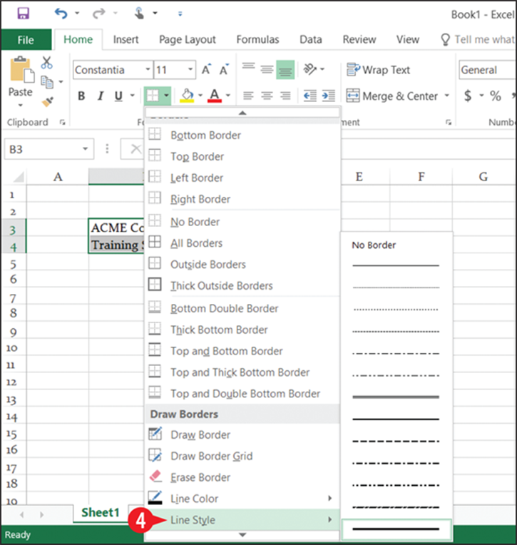
Figure 9-14: Select a line style.

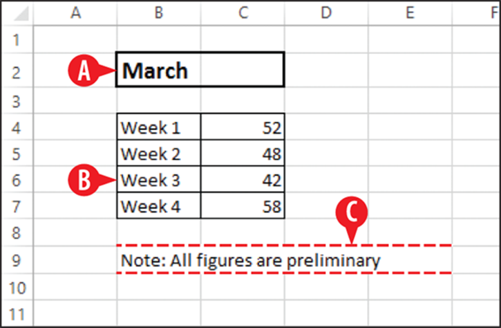
Figure 9-15: Some border examples.

Format cells using cell styles

As you learned in Chapter 3, in Word you can apply formatting preset called styles to individual paragraphs. You can do the same thing to individual cells in Excel, except in Excel they are called cell styles.

Excel provides a number of styles with names that reflect their suggested uses. For example, there are Heading 1 and Heading 2 styles, a Total style, and a Title style. There are also styles that apply shading using the theme’s color placeholders.

To apply a cell style to one or more cells:

Select the cell(s) to affect.

On the Home tab, click Cell Styles.

Click the desired style.

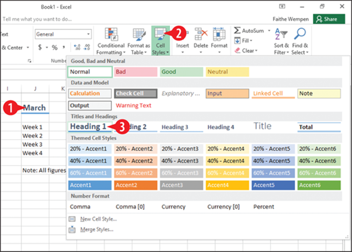
Figure 9-16: Apply a cell style.

You can also create your own custom cell styles. To do so:

Format a cell the way you want it, with font, color, alignment, border, and fill settings. Make sure that cell is selected.

On the Home tab, click Cell Styles.

Click New Cell Style.

Type a name for the style in the Style name box.

Review the style definition in the six categories listed.

If there is any additional formatting you need to define for the style, click Format. Make your choices in the Format Cells dialog box and click OK to return to the Style dialog box.

Click OK to create the style.

After you have defined a custom style, it appears at the top of the Cell Styles button’s gallery, in the Custom group. (See in Figure 9-19.)

To manage a custom style (modify, delete, or duplicate it), right-click it and choose the appropriate command. (See in Figure 9-19.)

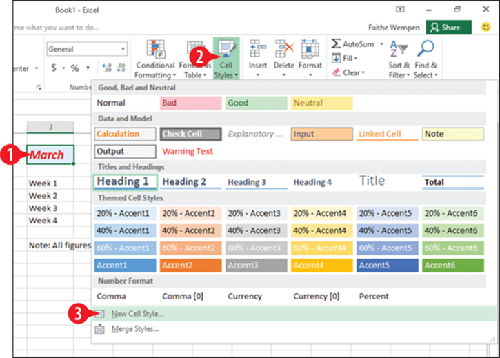
Figure 9-17: Format a cell the way you want the style, and then choose New Cell Style.

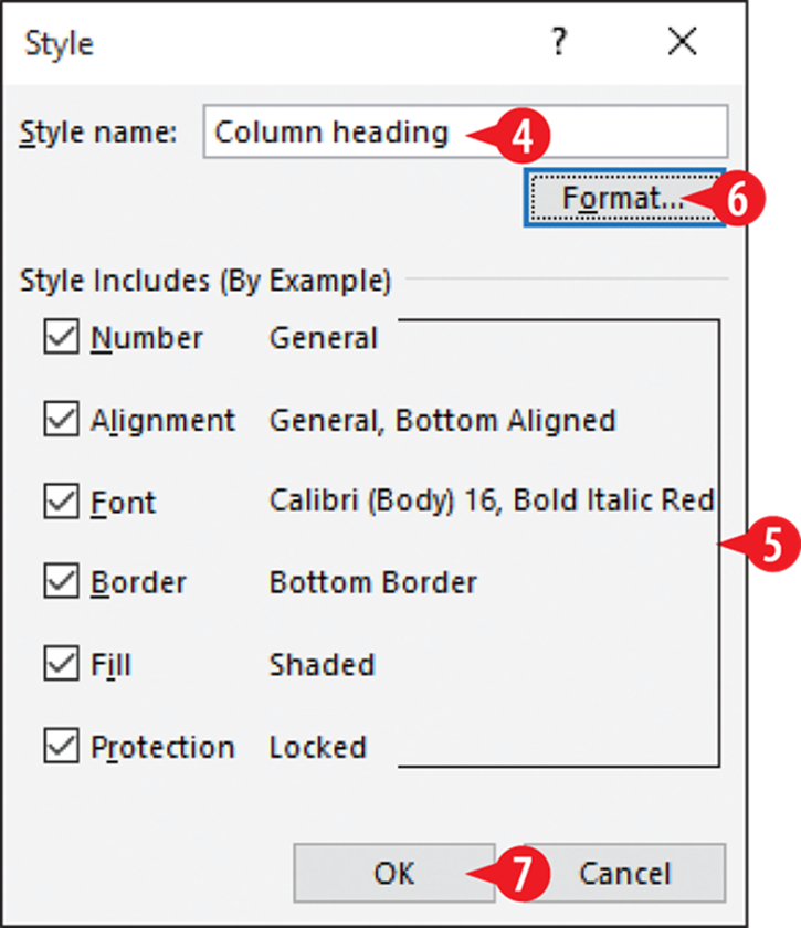
Figure 9-18: Define the new style with six categories of formatting.

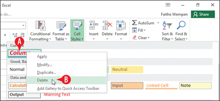
Figure 9-19: Custom styles appear at the top of the Cell Styles gallery.

Resize rows and columns

Each column in a worksheet starts with the same width, which is 8.43 characters (based on the default font and font size) unless you’ve changed the default setting. That’s approximately seven digits and either one large symbol (such as $) or two small ones (such as decimal points and commas).

You can define the default width setting for new worksheets: Choose Home  ⇒  Format  ⇒  Default Width and then fill in the desired default width.

As you enter data into cells, those column widths may no longer be optimal. Data may overflow out of a cell if the width is too narrow, or there may be excess blank space in a column if its width is too wide. (Blank space is not always a bad thing, but if you’re trying to fit all the data on one page, for example, it can be a hindrance.)

In some cases, Excel makes an adjustment for you automatically, as follows:

· For column widths: When you enter numbers in a cell, Excel widens a column as needed to accommodate the longest number in that column, provided you haven’t manually set a column width for it.

· For row heights: Generally, a row adjusts automatically to fit the largest font used in it. You don’t have to adjust row heights manually to allow text to fit. You can change the row height if you want, though, to create special effects, such as extra blank space in the layout.

The units of measurement are different for rows versus columns, by the way. Column width is measured in characters of the default font size. Row height is measured in points. A point is of an inch.

Change a row’s height

There may be times when you want to manually adjust a row’s height. For example, you might want to add some extra blank space vertically between one row’s text and another’s.

After you manually resize a row’s height or a column’s width, it won’t change its size automatically for you anymore. That’s because manual settings override automatic ones.

To manually change row height to a specific value, do the following:

1. Select any cell in the row.

Choose Format  ⇒  Row Height to open the Row Height dialog box.

Enter the desired row height in points. You can use decimal points for precise sizing if needed.

Click OK.

You can also adjust a row’s height manually by dragging the divider below the row’s number up or down. (See in Figure 9-22.)

A ScreenTip shows the height as you are dragging. (See in Figure 9-22.)

If you manually adjust a row height, that row will no longer autofit its height to content. To autofit row height, double-click the divider below the row’s number. (See in Figure 9-22.)

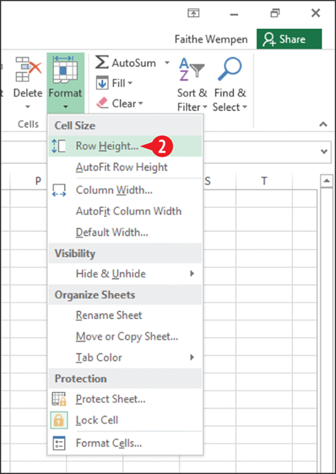
Figure 9-20: Choose Row Height from the menu.

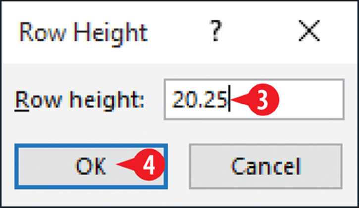
Figure 9-21: Specify a row height.

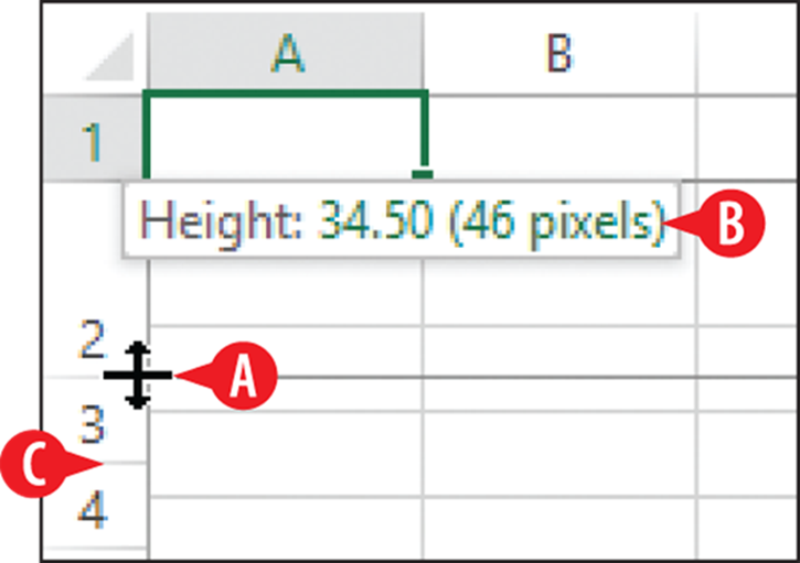
Figure 9-22: Adjust row height by dragging.

Change a column’s width

You can adjust a column width any time you need it to be wider or narrower to achieve the look you want. Most often this will be because the content of one or more cells in the column overflows its cell (or is truncated), but you can also widen or narrow columns to create specific layout effects, such as adding more space between columns of text or numbers.

To manually change column width to a specific value, do the following:

1. Select any cell in the row.

Choose Format  ⇒  Column Width to open the Column Width dialog box.

Enter the desired column width in characters (of the default font and size).

Click OK.

To autofit a column’s width to the widest entry in that column, double-click the divider below the column’s letter and the one to its right.

You can also adjust a column’s width manually by dragging the divider to the right of the column’s letter to the left or right. (See in Figure 9-25.)

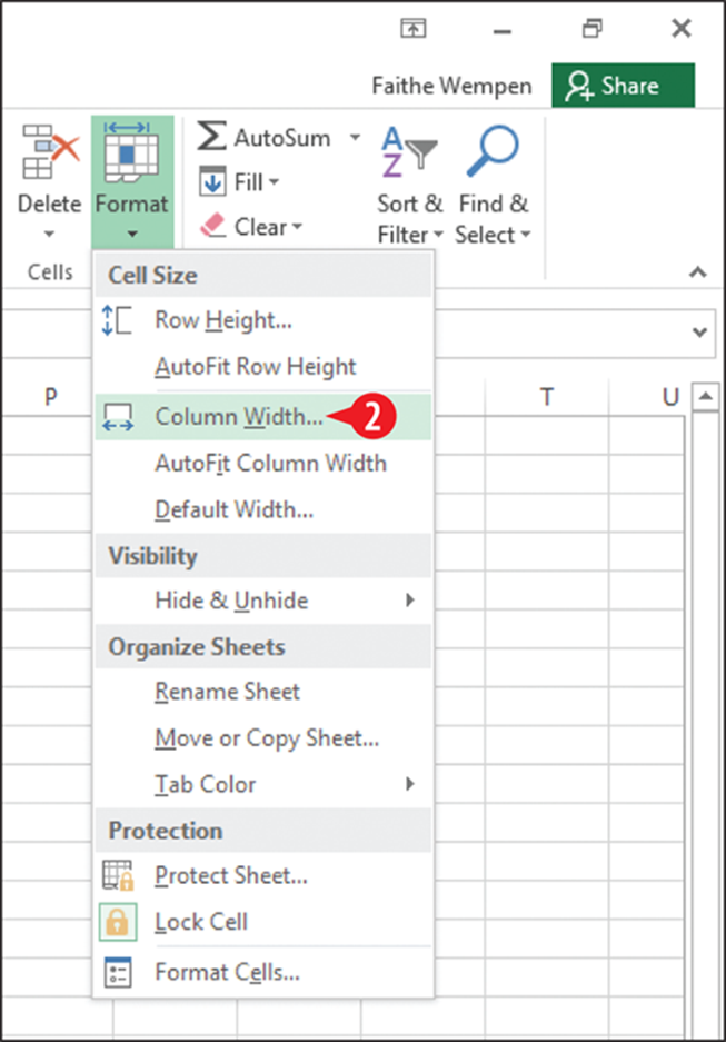
Figure 9-23: Choose Column Width from the menu.

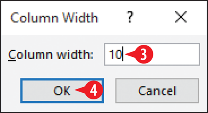
Figure 9-24: Specify a column width.

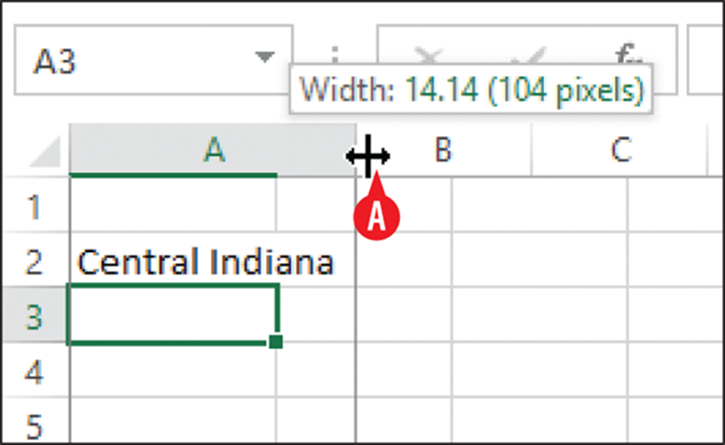
Figure 9-25: Adjust column width by dragging.

Make text wrap in a cell

When you have an entry that overflows its cell but you don’t want to widen the column for some reason (perhaps it would interfere with the worksheet’s layout, for example), you might choose to wrap the text in that cell to multiple lines. The row height increases automatically as much as needed to display the multiple lines and decreases again later if conditions change such that the additional height is no longer needed.

To wrap text in a cell:

1. Select the cell(s) that should be set for wrapping. You can set a cell for text wrapping even if it doesn’t have anything in it at the moment that requires wrapping.

On the Home tab, click Wrap Text.

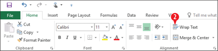
Figure 9-26: Wrap text to multiple lines in a cell.

To remove the setting for a cell (or multiple cells), repeat the steps to toggle the option off.

Use conditional formatting

Conditional formatting is formatting that appears only if certain conditions are met in the cell’s content. It can help readers understand the data they are seeing more easily. For example, you might have a cell display a green background if the value is over a certain amount and a red background if the value is under a certain amount. A reader can quickly scan a long column of numbers and zero in on just the red or green shaded cells as being especially small or large.

Excel provides several preset types of conditional formatting, including these:

· Data bars: Each cell has left-to-right shading proportionate to the value of the number. The end result is that each cell functions as a mini-chart. See Figure 9-27 for an example.

· Color scales: Each cell has a background color that reflects its content. For example, in Figure 9-28, lower numbers are red, average numbers are yellow, and higher numbers are green.

· Icon sets: Each cell has an icon that varies depending on its content. In Figure 9-29, higher numbers have green check marks, average numbers have yellow exclamation points, and lower numbers have red Xs.

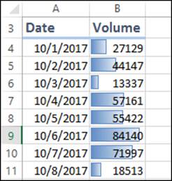
Figure 9-27: Data bars.

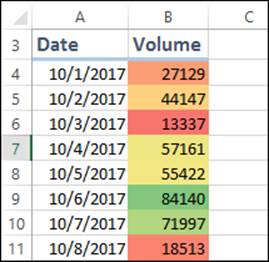
Figure 9-28: Color scale.

You can also define your own custom conditional formatting.

Apply conditional formatting

Let’s look at a simple example: applying a color scale. In the following steps you will apply a preset color scale and then customize it.

1. Select the cells to which to apply conditional formatting.

On the Home tab, click Conditional Formatting.

Point to Color Scales.

Click the desired color scale—or one that is close to what you want if none are right.

Next, you’ll customize the preset that you just applied.

With the same range still selected, click Conditional Formatting again.

Click Manage Rules.

Select the rule you just created.

Click Edit Rule.

Open the Color palette under Minimum and choose the desired color.

Open the Color palette under Maximum and choose the desired color.

Change any other aspects of the rule as desired. For example, you can define exact minimum and maximum values, change the midpoint, choose more or fewer colors for the scale, and so on.

Click OK.

13. Click OK to close the Conditional Formatting Rules Manager.

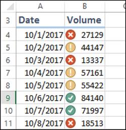
Figure 9-29: Icon set.

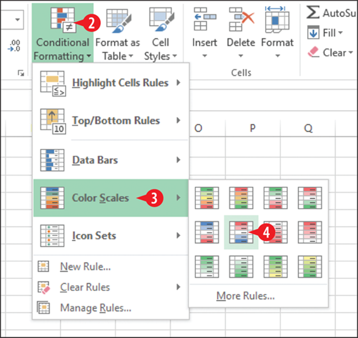
Figure 9-30: Choose a conditional formatting preset.

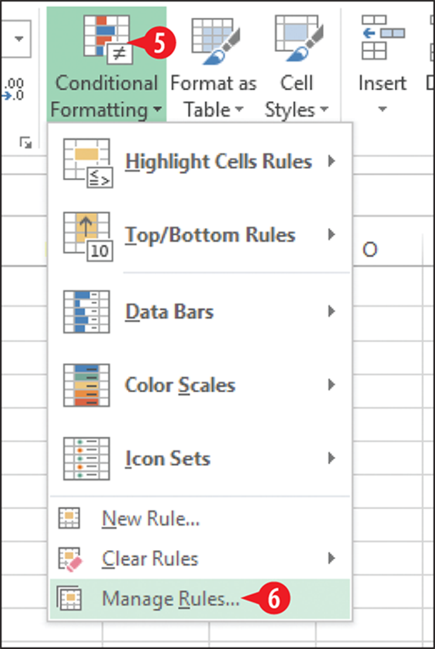
Figure 9-31: Choose Manage Rules.

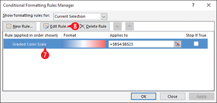
Figure 9-32: Select the rule to edit.

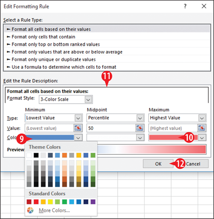
Figure 9-33: Modify the rule.

Remove conditional formatting

To remove the conditional formatting from cells:

1. Select the cells from which to remove conditional formatting.

On the Home tab, click Conditional Formatting.

Point to Clear Rules.

Click Clear Rules from Selected Cells.

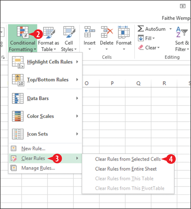
Figure 9-34: Clear conditional formatting.

Set up headers and footers

If you plan to print your worksheet, you might want to set up a header and/or footer. Headers and footers are lines of information that repeat at the top and bottom of each page. These lines can contain any text you want plus codes that print page numbers, the current date and time, or other information.

The header and footer areas exist on all worksheets, but by default they are blank so you don’t notice them. Follow these steps to display the header and footer areas and place text and codes in them as desired:

On the Insert tab, click Header & Footer.

The display changes to Page Layout view. The worksheet is displayed as it will print, with header and footer areas at the top and bottom. Consider Figure 9-36:

Notice that the Header area consists of three boxes. Depending on which box you choose to enter content into, it will appear left-aligned, centered, or right-aligned at the top of the page.

The Header & Footer Tools Design tab appears, containing buttons for inserting various types of content into the header and footer.

(Optional) If you want to work with the footer, click Go to Footer.

Click in the placeholder area in which you want to enter header or footer content. The insertion point appears in it.

If you want text to appear, type it. Any text you type will appear the same on all pages.

Click to move the insertion point to a different section if desired.

6. Click a button on the Header & Footer Tools Design tab to insert a code:

Page Number shows the page number of each printed page.

Number of Pages shows the total number of pages in the printout.

You might want to type of between the Page Number and Number of Pages codes.

Current Date inserts an automatically updating date code.

Current Time inserts an automatically updating time code.

File Path prints the entire path and file name of the workbook.

File Name prints only the file name (not the path) of the workbook.

Sheet Name prints the sheet name (as represented on the sheet tab).

Picture prompts you to select a picture to include. Note that this picture will not be confined to the header or footer area.

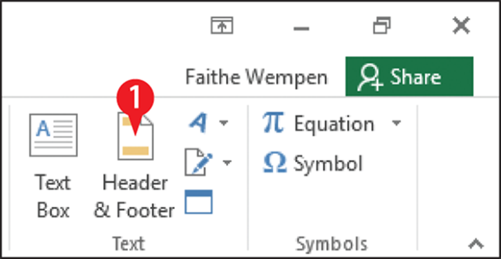
Figure 9-35: Choose Header & Footer from the Insert tab.

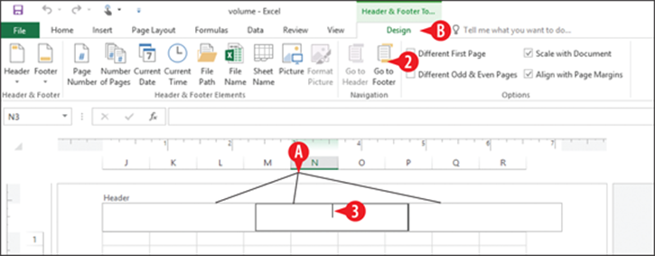
Figure 9-36: The Header area in Page Layout view.

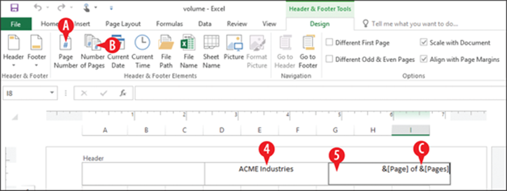
Figure 9-37: Codes inserted in a header.

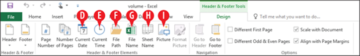
Figure 9-38: Other types of codes you can insert.

The Picture code is somewhat different from the other codes. You are prompted for the picture to use when you insert this code. You can choose a picture from your own files, or you can search online for a picture.

Depending on its size, the picture may overflow out of the header and footer, into the background of the worksheet itself. The picture starts out in whatever area of the header or footer you place it in. So, for example, if you want a picture to start in the lower right corner of the page and extend upward and to the left from there, place its code in the right-hand section of the footer.

To change the picture’s size, click Format Picture. In the Format Picture dialog box, on the Size tab, you can set its height and width. You can also crop the picture using the controls on the Picture tab of that dialog box.

If you don’t see the picture immediately after inserting the code, click in some other section of the header or footer to move the insertion point out of the one where the picture code resides, and the picture should appear.

Print a worksheet

You can print your work in Excel on paper to share with people who may not have computer access or to pass out as handouts at meetings and events. You can print the quick-and-easy way with the default settings or customize the settings to fit your needs.

By default, when you print, Excel prints the entire active worksheet — that is, whichever worksheet is displayed or selected at the moment. But Excel also gives you other printing options:

· Print multiple worksheets: If more than one worksheet is selected (for example, if you have more than one worksheet tab selected at the bottom of the Excel window), all selected worksheets are included in the printed version. As an alternative, you can print all the worksheets in the workbook. To select more than one worksheet, hold down the Ctrl key as you click the tabs of the sheets you want.

· Print selected cells or ranges: You can choose to print only selected cells, or you can define a print range and print only that range (regardless of what cells happen to be selected).

Print entire worksheets

To print the active worksheet, and optionally other worksheets too in the same workbook, follow these steps:

If you want to print only one worksheet, click its tab to make sure it is active.

OR

If you want to print multiple worksheets, hold down Ctrl and click each of the worksheet tabs of the desired sheets to group them.

Choose File  ⇒  Print.

If you chose more than one sheet in step 1, [Group] appears in the title bar. (See in Figure 9-40.)

Make sure the correct printer appears in the Printer setting; click to change it if needed.

Specify a number of copies in the Copies box.

Change any additional print settings as needed. For example, you can change the collation options if you are printing multiple copies, and you can change the margins and paper size. These options are like the ones you learned about in “Print your work” in Chapter 2.

(Optional) Click the left and right arrows to preview the pages of the print job.

Click Print.

8. If you grouped sheets in step 1, right-click one of the grouped sheet tabs and choose Ungroup Sheets.

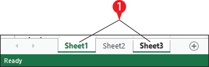
Figure 9-39: Select the tabs of the sheets to print, if more than one.

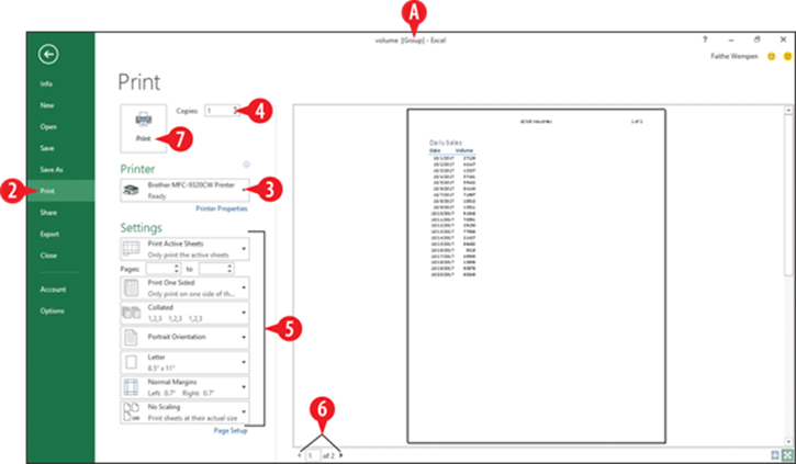
Figure 9-40: Set print options and then click Print.

Set and use a print range

If you want to select a range for a one-time print job, you can select the range of cells and then choose to print only the selection. Here’s how:

1. Select the cells to print.

2. Choose File  ⇒  Print.

Click Print Active Sheets to open a menu.

Click Print Selection.

5. Continue printing normally, as in the previous section’s steps.

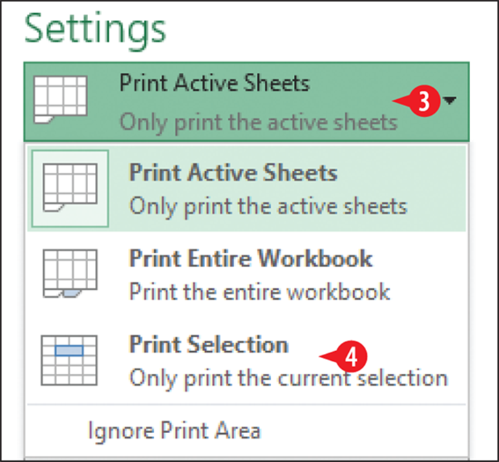
Figure 9-41: Choose to print only the selected cells.

If you want to print a certain range every time you print that sheet, it may make more sense to set a print range. When you do so, Excel prints only the cells included in your specified range, even when you don’t select that range before printing.

To set a print range:

1. Select the desired cells to include.

On the Page Layout tab, click Print Area.

Click Set Print Area.

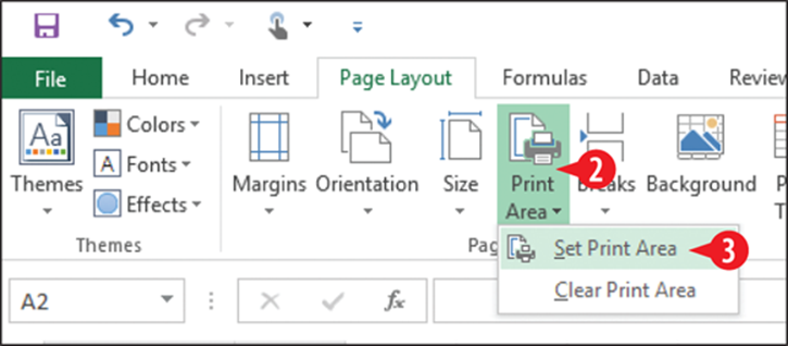
Figure 9-42: Set the print area.

When a print area is set, nothing outside of that area will print on that sheet. If you want to override this behavior temporarily to print the entire sheet, choose the Ignore Print Area command on the menu shown in Figure 9-41.

To clear the print area, repeat the steps for setting the print area, but in step 3 choose Clear Print Area instead.

If you want the same cells (only) to print each time you print this worksheet in the future too, you can select them as a print range, and Excel remembers them.