My Office 2016 (2016)
8. Visualizing Excel Data with Charts
In this chapter, you learn about creating, customizing, and formatting charts to help visualize your Excel data. Topics include the following:
![]() Converting Excel data into a chart
Converting Excel data into a chart
![]() Working with Excel’s different chart types
Working with Excel’s different chart types
![]() Moving, resizing, and changing the layout of a chart
Moving, resizing, and changing the layout of a chart
![]() Selecting and formatting chart elements
Selecting and formatting chart elements
![]() Adding chart titles, a legend, and data labels
Adding chart titles, a legend, and data labels
One of the best ways to analyze your worksheet data—or get your point across to other people—is to display your data visually in a chart. Excel gives you tremendous flexibility when creating charts: It enables you to place charts in separate documents or directly on the worksheet itself. Not only that, but you have dozens of different chart formats to choose from, and if none of Excel’s built-in formats is just right, you can further customize these charts to suit your needs.
Creating a Chart
When plotting your worksheet data, you have two basic options: You can create an embedded chart that sits on top of your worksheet and can be moved, sized, and formatted; or you can create a separate chart sheet. Whether you choose to embed your charts or store them in separate sheets, the charts are linked with the worksheet data. Any changes you make to the data are automatically updated in the chart.
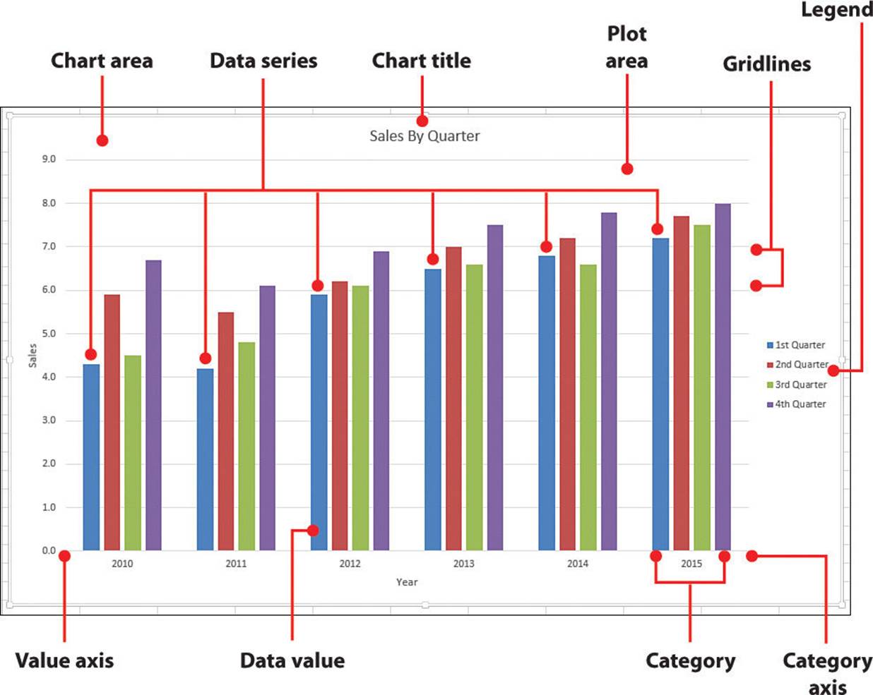
Before getting to the specifics of creating a chart, you should familiarize yourself with some basic chart terminology:
• Category—A grouping of data values on the category horizontal axis.
• Category axis—The axis (usually the x-axis) that contains the category groupings.
• Chart area—The area on which the chart is drawn.
• Data marker—A symbol that represents a specific data value. The symbol used depends on the chart type. In a column chart, for example, each column is a marker.
• Data series—A collection of related data values. Normally, the marker for each value in a series has the same pattern.
• Data value—A single piece of data. Also called a data point.
• Gridlines—Optional horizontal and vertical extensions of the axis tick marks. These make data values easier to read.
• Legend—A guide that shows the colors, patterns, and symbols used by the markers for each data series.
• Plot area—The area bounded by the category and value axes. It contains the data points and gridlines.
• Tick mark—A small line that intersects the category axis or the value axis. It marks divisions in the chart’s categories or scales.
• Value axis—The axis (usually the y-axis) that contains the data values.
Create an Embedded Chart
An embedded chart is one that appears on the same worksheet as the data that it’s based on. Creating an embedded chart is by far the easiest way to build a chart in Excel because the basic technique requires just a few steps.
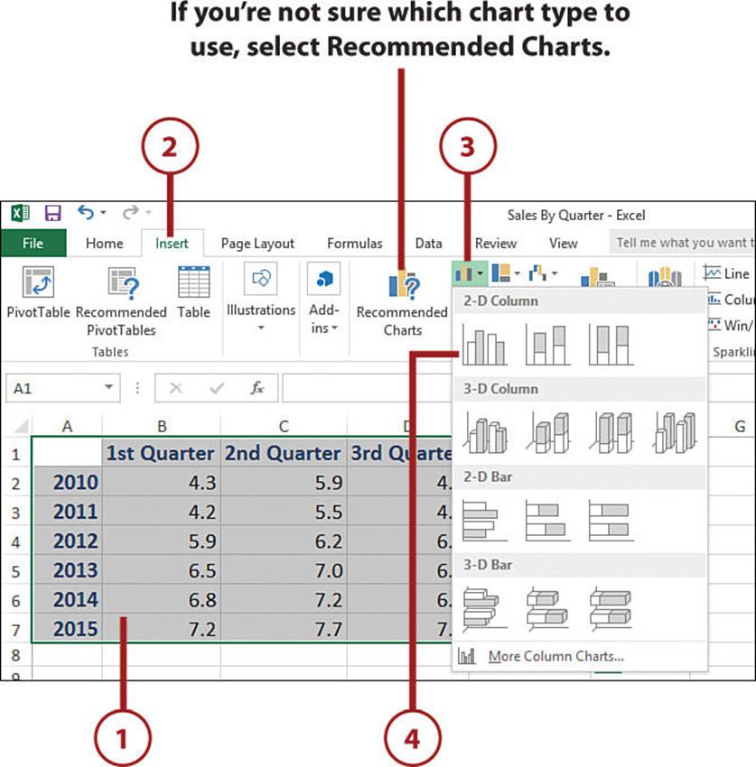
1. Select the range you want to plot, including the row and column labels if there are any. Make sure that no blank rows are between the column labels and the data.
2. Select Insert.
3. In the Charts group, drop down the list for the chart type you want. Excel displays a gallery of chart types.
4. Select a chart type. Excel embeds the chart.
Create a Chart in a Separate Sheet
If you don’t want a chart taking up space in a worksheet, or if you want to print a chart on its own, you can create a separate chart sheet.
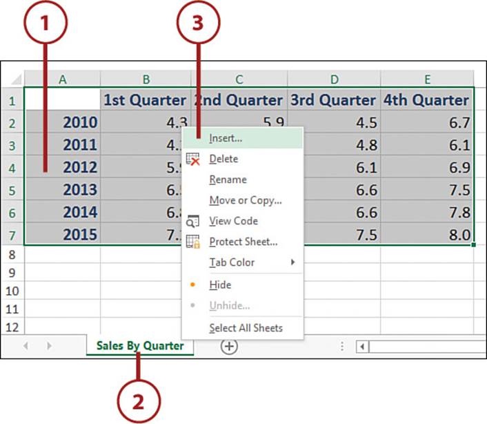
1. Select the range you want to plot, including the row and column labels if there are any. Make sure that no blank rows are between the column labels and the data.
2. Right-click the tab of the worksheet before which you want the chart sheet to appear.
3. Select Insert. Excel displays the Insert dialog box.
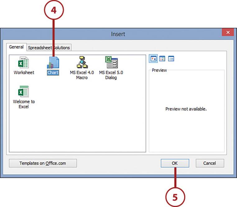
4. Select Chart.
5. Select OK. Excel creates the chart sheet and adds a default chart.
Keyboard Shortcut
To insert a chart in a separate sheet using the keyboard, select the data you want to chart and then press F11.
Working with Charts
Once you’ve created a chart, Excel offers various tools for working with the chart, including changing the chart type, moving and resizing the chart, and changing the chart layout. The next few sections provide the details.
Understanding Excel’s Chart Types
To help you choose the chart type that best presents your data, the following list provides brief descriptions of all of Excel’s chart types:
• Area chart—An area chart shows the relative contributions over time that each data series makes to the whole picture. The smaller the area a data series takes up, the smaller its contribution to the whole.
• Bar chart—A bar chart compares distinct items or shows single items at distinct intervals. A bar chart is laid out with categories along the vertical axis and values along the horizontal axis. This format lends itself to competitive comparisons because categories appear to be “ahead” or “behind.”
• Bubble chart—A bubble chart is similar to an XY chart, except that it uses three data series, and in the third series the individual plot points are displayed as bubbles (the larger the value, the larger the bubble).
• Box & Whisker chart—Visualizes several statistical values for the data in each category, including the average, range, minimum, and maximum.
• Column chart—Like a bar chart, a column chart compares distinct items or shows single items at distinct intervals. However, a column chart is laid out with categories along the horizontal axis and values along the vertical axis (as are most Excel charts). This format is best suited for comparing items over time. Excel offers various column chart formats, including stacked columns. A stacked column chart is similar to an area chart; series values are stacked on top of each other to show the relative contributions of each series. Although an area chart is useful for showing the flow of the relative contributions over time, a stacked column chart is better for showing the contributions at discrete intervals.
• Doughnut chart—A doughnut chart, like a pie chart, shows the proportion of the whole that is contributed by each value in a data series. The advantage of a doughnut chart, however, is that you can plot multiple data series. (A pie chart can handle only a single series.)
• Histogram—Groups the category values into ranges, called bins, and shows the frequency with which the data values fall within each bin.
• Line chart—A line chart shows how a data series changes over time. The category (x) axis usually represents a progression of even increments (such as days or months), and the series points are plotted on the value (y) axis. Excel offers several stock chart formats, including an Open, High, Low, Close chart (also called a candlestick chart), which is useful for plotting stock-market prices.
• Pie chart—A pie chart shows the proportion of the whole that is contributed by each value in a single data series. The whole is represented as a circle (the “pie”), and each value is displayed as a proportional “slice” of the circle.
• Radar chart—A radar chart makes comparisons within a data series and between data series relative to a center point. Each category is shown with a value axis extending from the center point. To understand this concept, think of a radar screen in an airport control tower. The tower itself is the central point, and the radar radiates a beam (a value axis). When the radar makes contact with a plane, a blip appears onscreen. In a radar chart, this data point is shown with a data marker.
• Sunburst chart—Displays hierarchical data as a series of concentric circles, with the top level as the innermost circle and each circle divided proportionally according to the data values within that level.
• Treemap chart—For hierarchical data, shows a large rectangle for each item in the top level, and then divides each rectangle proportionally based on the value of each item in the next level.
• Waterfall chart—Shows a running total as category values are added (positive values) or subtracted (negative values).
• XY (scatter) chart—An XY chart (also called a scatter chart) shows the relationship between numeric values in two different data series. It also can plot a series of data pairs in x,y coordinate. An XY chart is a variation of the line chart in which the category axis is replaced by a second value axis. You can use XY charts for plotting items such as survey data, mathematical functions, and experimental results.
• 3-D charts—In addition to the various 2-D chart types presented so far, Excel also offers 3-D charts. Because they’re striking, 3-D charts are suitable for presentations, flyers, and newsletters. (If you need a chart to help with data analysis, or if you just need a quick chart to help you visualize your data, you’re probably better off with the simpler 2-D charts.) Most of the 3-D charts are just the 2-D versions with an enhanced 3-D effect. However, some 3-D charts enable you to look at your data in new ways. For example, some 3-D area chart types enable you to show separate area plots for each data series (something a 2-D area chart can’t do). In this variation, the emphasis isn’t on the relative contribution of each series to the whole; rather, it’s on the relative differences among the series.
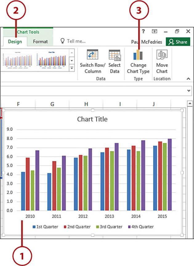
Change the Chart Type
If you feel that the current chart type is not showing your data in the best way, you can change the chart type. This enables you to experiment not only with the 10 different chart types offered by Excel, but also with its nearly 100 chart type configurations.
1. Select the chart.
2. Select the Design tab.
3. Select Change Chart Type. The Change Chart Type dialog box opens.
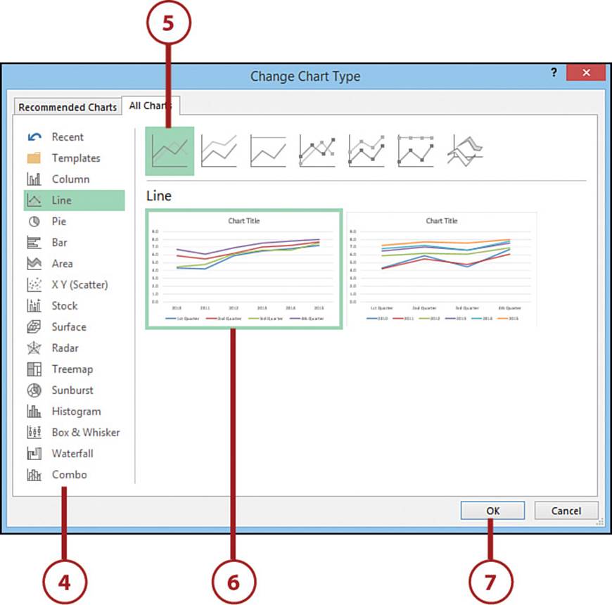
4. Select the chart type you want to use. Excel displays the chart type configurations.
5. Select the general configuration you want to use.
6. Select the specific configuration you want to use.
7. Select OK.
>>>Go Further: Creating a Chart Template
Once you’ve changed the chart type, as described in this section, and performed other chart-related chores such as applying titles, adding labels, and choosing a layout (described later in this chapter), you might want to repeat the same settings on another chart. Rather than repeating the same procedures on the second chart, you can make your life easier by saving the original chart as a chart template. This enables you to then build the second chart (and any subsequent charts) based on this template. To save the chart as a template, right-click the chart’s plot area or background and then select Save as Template. Type a name for the template and then select Save. To reuse the template, follow steps 1 to 3 in this section, select Templates, select your template, and then select OK.
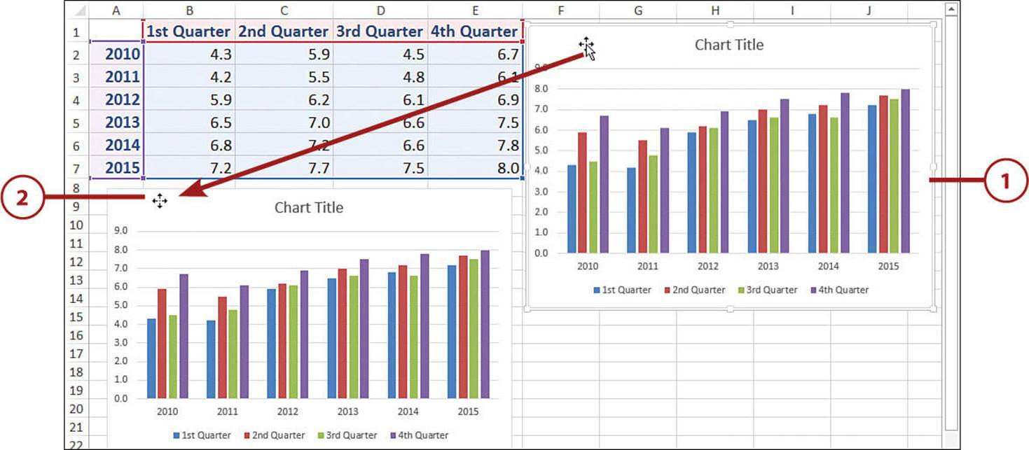
Move a Chart
You can move a chart to another part of the worksheet. This is useful if the chart is blocking the worksheet data or if you want the chart to appear in a particular part of the worksheet.
1. Click the chart to select it.
2. Click and drag an empty section of the chart to the location you want. As you drag, Excel moves the chart.
Dragging an Edge
If you drag a chart object such as the plot area or the chart title, you’ll only move that object, not the entire chart. If you’re having trouble finding a place to drag, try dragging any edge of the chart. However, try to avoid dragging any of the selection handles (see the next section), or you’ll just resize the chart.
>>>Go Further: Moving a Chart to a Separate Sheet
In the “Create a Chart in a Separate Sheet” section, earlier in this chapter, you learned how to create a new chart in a separate sheet. If your chart already exists on a worksheet, you can move it to a new sheet. Click the chart, select the Design tab, and then select Move Chart to open the Move Chart dialog box. Select the New Sheet option, use the New Sheet text box to type a name for the new sheet, and then select OK.
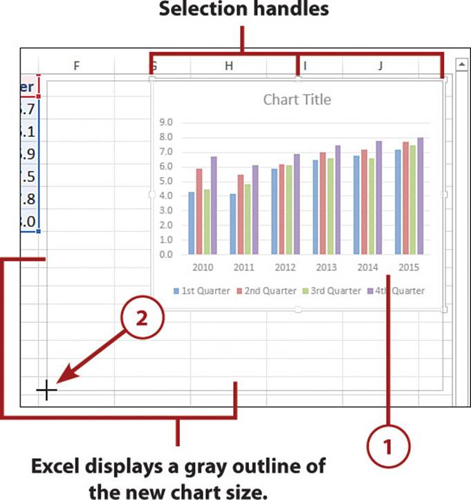
Resize a Chart
You can resize a chart. For example, if you find that the chart is difficult to read, making the chart bigger often solves the problem. Similarly, if the chart takes up too much space on the worksheet, you can make it smaller.
1. Click the chart. Excel displays a border around the chart, which includes selection handles on the corners and sides.
2. Click and drag a selection handle until the chart is the size you want. When you release the screen, Excel resizes the chart.
Change the Chart Layout and Style
You can quickly format your chart by applying a different chart layout. The chart layout includes elements such as the titles, data labels, legend, and gridlines. The Quick Layouts feature in Excel enables you to apply these elements in different combinations in just a few steps. You can also apply a chart style, which governs the formatting applied to the chart background, data markers, gridlines, and more.
1. Click the chart.
2. Select the Design tab.
3. Select Quick Layout.
4. Select the layout you want to use.
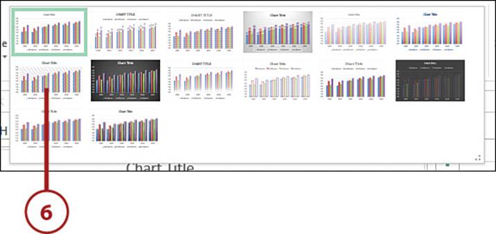
5. Select the More button in the Chart Styles section. Excel displays the Chart Styles gallery.
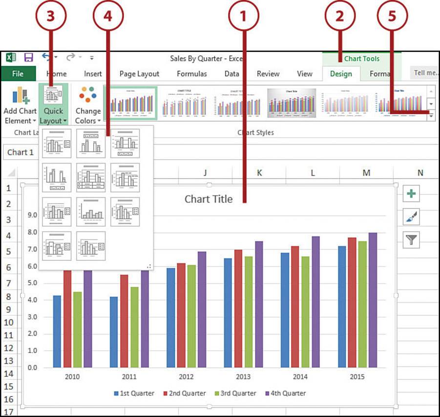
6. Select the style you want to apply.
Working with Chart Elements
An Excel chart is composed of elements such as axes, data markers, gridlines, and text, each with its own formatting options. In the rest of this chapter, you learn how to work with several of these elements, including titles, legends, and data markers.
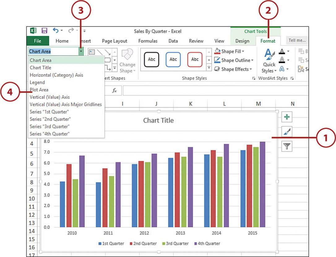
Select Chart Elements
Before you can format a chart element, you need to select it.
1. Click the chart.
2. Select the Format tab.
3. Drop down the Chart Elements list to display a list of all the elements in the current chart.
4. Select the element you want to work with.
Selecting Chart Elements Directly
You can also select many chart elements directly by clicking them.
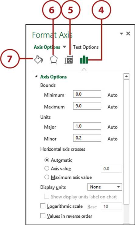
Format Chart Elements
If you want to format a particular chart element, the Format tab offers several options for most chart elements. However, the bulk of your element formatting chores will take place in the Format task pane, the layout of which depends on the selected element.
1. Select the chart element you want to format.
2. Select the Format tab.
3. Select Format Selection. Excel displays the Format task pane.

4. Select the Options tab to work with the element’s settings.
5. Select the Size & Properties tab to control the size of the element and set the element’s properties.
6. Select the Effects tab to control element formatting such as shadows, glow effects, soft edges, and 3-D effects.
7. Select the Fill & Line tab to control formatting such as the element’s background color and the color and style of its borders.
Format Task Pane Tabs
Not all chart elements display all the tabs mentioned here.
Add Titles
Excel enables you to add four kinds of titles: the chart title is the overall chart title, and you use it to provide a brief description that puts the chart into context; the category (X) axis title appears below the category axis, and you use it to provide a brief description of the category items; thevalue (Y) axis title appears to the left of the value axis, and you use it to provide a brief description of the value items; and the value (Z) axis title appears beside the z-axis in a 3-D chart, and you use it to provide a brief description of the z-axis items.
1. Click the chart.
2. Select the Design tab.
3. Select Add Chart Element.
4. Select Chart Title.
5. Select Above Chart. Excel adds the title box.
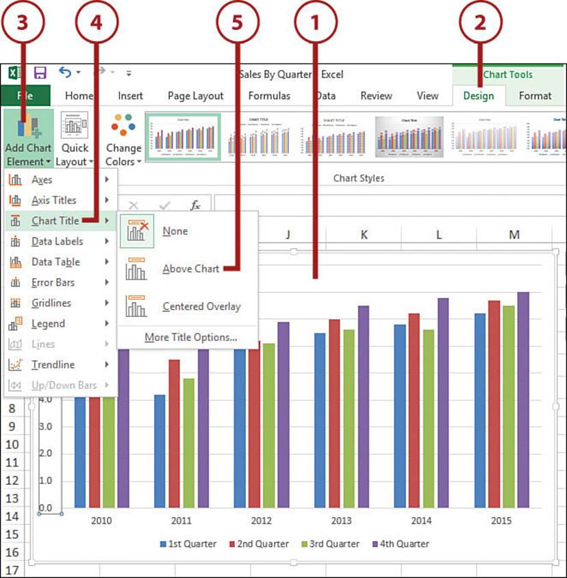
6. Type the title.
7. Select Add Chart Element.
8. Select Axis Titles.
9. Select Primary Horizontal. Excel adds the title box.
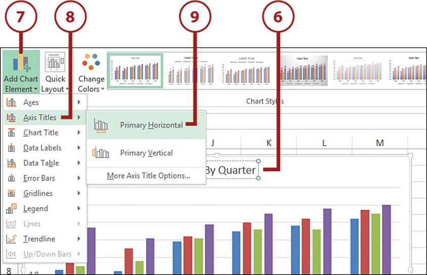
10. Type the title.
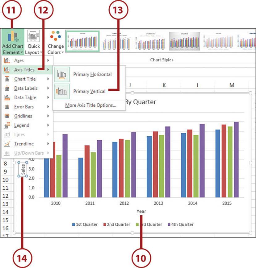
11. Select Add Chart Element.
12. Select Axis Titles.
13. Select Primary Vertical. Excel adds the title box.
14. Type the title.
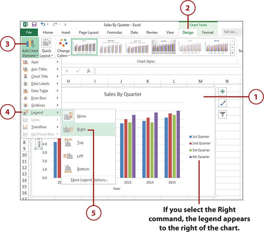
Add a Chart Legend
If your chart includes multiple data series, you should add a legend to explain the series markers. Doing so makes your chart more readable and makes it easier for others to distinguish each series.
1. Click the chart.
2. Select the Design tab.
3. Select Add Chart Element.
4. Select Legend.
5. Select the position you want to use for the legend. Excel adds the legend.
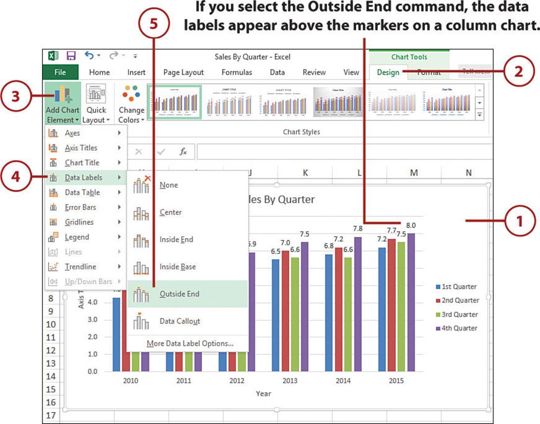
Add Data Marker Labels
You can make your chart easier to read by adding data labels. A data label is a small text box that appears in or near a data marker and displays the value of that data point.
1. Click the chart.
2. Select the Design tab.
3. Select Add Chart Element.
4. Select Data Labels.
5. Select the position you want to use for the data labels. Excel adds the labels to the chart.
Data Label Positions
The data label position options you see depend on the chart type. For example, with a column chart you can place the data labels within or above each column, and for a line chart you can place the labels to the left or right, or above or below, the data marker.
All materials on the site are licensed Creative Commons Attribution-Sharealike 3.0 Unported CC BY-SA 3.0 & GNU Free Documentation License (GFDL)
If you are the copyright holder of any material contained on our site and intend to remove it, please contact our site administrator for approval.
© 2016-2026 All site design rights belong to S.Y.A.